


")


")

")
")
 in Excel & Google Sheets")


The UNIQUE function doesn’t inherently include only visible rows when it returns values, discarding duplicates in Google Sheets.
However, we can utilize a workaround method to achieve the desired result involving the MAP lambda function.
The logic is as follows: We will first identify visible rows and use the FILTER function to extract them. Then we apply the UNIQUE function to the extracted range.
Below, you will find step-by-step instructions for applying the UNIQUE function to visible rows in Google Sheets.
Sample Data and Testing Default Behavior of UNIQUE in a Filtered Range
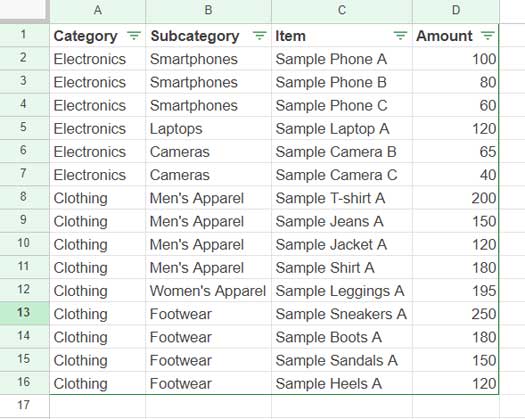
The sample data is in A1:D16, where A1:D1 contains the field labels.
There are two unique categories in A2:A16, i.e., Electronics and Clothing, which we can extract using the following UNIQUE formula:
=UNIQUE(A2:A16)Let’s filter out one of the categories, which is Electronics, and see what the formula returns.
For that, select A1:D16 and click Data > Create a Filter.
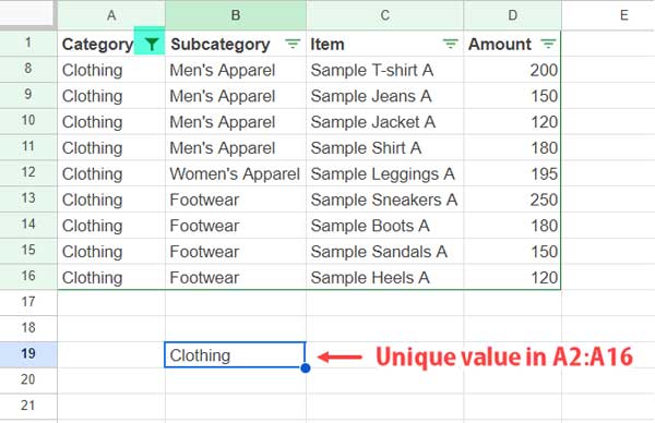
Click the filter drop-down in cell A1, uncheck Electronics, and click OK.
Now, there is only one visible category, which is Clothing. However, the above UNIQUE formula will still return the same two unique categories.
The proper way to apply the UNIQUE function to visible rows in Google Sheets is here.
Step-by-Step Instructions for Using the UNIQUE Function in Visible Rows
To determine whether cell A2 is visible in Google Sheets, you can use the following SUBTOTAL formula:
=SUBTOTAL(103, A2)This formula outputs 0 if row #2 is hidden and 1 if it’s visible. Function #103 represents COUNTA in visible cells.
To apply this formula to each row in the range A2:A16, you need to convert it into a custom LAMBDA function.
The syntax for creating a custom lambda function is:
LAMBDA(name, formula_expression)Here’s the custom lambda function:
LAMBDA(r, SUBTOTAL(103, r))You can use this lambda function within the MAP function. The syntax for MAP is:
=MAP(array1, lambda)Where array1 is A2:A16.
=MAP(A2:A16, LAMBDA(r, SUBTOTAL(103, r)))In this lambda function, “r” represents the current element in the array. The MAP function iterates over each value in the array and returns 1 for visible rows and 0 for hidden rows.
Next, you can FILTER the range A2:A16 where the MAP output is 1. The syntax for FILTER is:
=FILTER(range, condition)Here is that FILTER formula:
=FILTER(A2:A16, MAP(A2:A16, LAMBDA(r, SUBTOTAL(103, r))))Here, the range is A2:A16, and the condition is the MAP formula.
Finally, wrap this formula with UNIQUE to get unique values in the visible rows:
=UNIQUE(FILTER(A2:A16, MAP(A2:A16, LAMBDA(r, SUBTOTAL(103, r)))))