How to Use the STDEVA Function in Google Sheets

The STDEVA function in Google Sheets is used to calculate the standard deviation of a sample, including numbers, text, and logical values (TRUE/FALSE). It’s particularly useful when you want to measure how much variation or dispersion exists in a dataset — for example, to assess the volatility of an investment.

A smaller standard deviation (SD) indicates that values are closer to the average (mean), suggesting stability. A larger standard deviation means greater fluctuation. If the SD is 0, it means there’s no variability at all.

Why Use STDEVA?

While STDEVA is often used in financial contexts — like tracking investment performance — it’s not limited to that.

For example, you can also use it to measure how the heights of trees in a forest deviate from the average. Essentially, it’s a statistical tool for understanding variation in sample data.

Standard Deviation Functions in Google Sheets

Google Sheets offers several functions to calculate the standard deviation of a sample:

STDEVA
STDEV
STDEV.S (the newer function that replaces STDEV)
DSTDEV
SUBTOTAL (using function number 7 or 107)

Some of these functions are designed for compatibility with other spreadsheet applications, while others are intended for specific use cases, such as working with filtered data or structured database-style ranges.

What Makes STDEVA Different?

The STDEVA function stands out because:

It includes text values (as 0)
It includes logical values: TRUE is treated as 1, FALSE as 0
Other standard deviation functions typically ignore these values

STDEVA Syntax

STDEVA(value1, [value2, ...])

value1: The first number, logical value, or range of the sample
value2, ...: Additional values or ranges to include

You need at least two values to calculate the standard deviation, or the function will return an error.

Examples of STDEVA in Google Sheets

Basic Example:

=STDEVA(5)

Returns: #DIV/0!
Explanation: Only one value provided — not enough for a sample SD.

With Three Numbers

=STDEVA(5, 10, 15)

✅ Returns: 5
This measures the spread of 5, 10, and 15 from their average (10).

Including Logical Value FALSE

=STDEVA(5, 10, 15, FALSE)

✅ Returns: 6.45
Since FALSE is treated as 0, it increases the spread.

Including Logical Value TRUE

=STDEVA(5, 10, 15, TRUE)

✅ Returns: 6.08
Here, TRUE is treated as 1.

Including Text Values

When passed as a cell reference, text values are treated as 0:

=STDEVA(A1:A5)

(If one of those cells contains text like “nil”, it’s counted as 0.)

But if you hardcode text into the formula:

=STDEVA(5, 10, "nil", 1)

Returns: #VALUE!
Explanation: Hardcoded text causes an error.

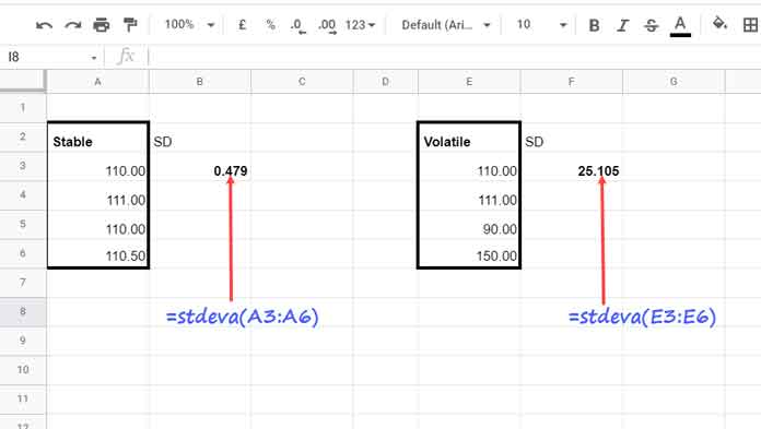
STDEVA Example: Volatile vs Stable Investment

Let’s compare two sample datasets:

Stable values in A3:A6 (e.g., 110, 111, 110, 110.5) — values are close to each other
Volatile values in E3:E6 (e.g., 110, 111, 90, 150) — values vary widely

=STDEVA(A3:A6)  → Returns: 0.479
=STDEVA(E3:E6)  → Returns: 25.1

This illustrates how standard deviation captures the spread of data — the higher the value, the more volatile or inconsistent the dataset.

Example showing how the STDEVA function in Google Sheets calculates standard deviation for stable vs. volatile investment values

Comparing STDEVA with Other Functions

When calculating the standard deviation of a sample, it’s important to understand the differences among functions.

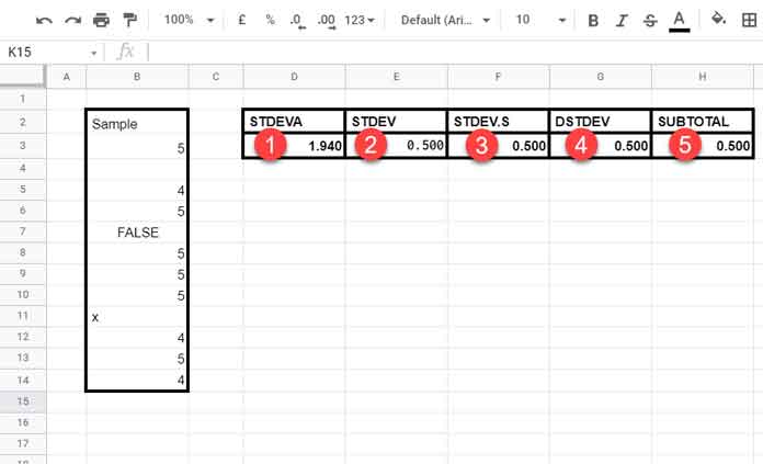
Comparison table of standard deviation functions in Google Sheets including STDEVA, STDEV, STDEV.S, DSTDEV, and SUBTOTAL with example formulas

1. `STDEVA`

=STDEVA(B3:B14)

Ignores blanks
Treats text and FALSE as 0, TRUE as 1

2. `STDEV`

=STDEV(B3:B14)

Ignores text and logical values

Compare with:

=STDEVA(FILTER(B3:B14, ISNUMBER(B3:B14)))

3. `STDEV.S`

=STDEV.S(B3:B14)

Identical to STDEV (alias for compatibility)

4. `DSTDEV` (Database function)

=DSTDEV(B2:B14, 1, {"Sample"; IF(,,)})

DSTDEV ignores text and Boolean values in the data range. It includes only numeric values that meet the specified criteria. This function is best suited for structured, database-style tables with labeled columns.

5. `SUBTOTAL` (Visible data only)

=SUBTOTAL(107, B3:B14)

SUBTOTAL calculates the standard deviation of visible numeric cells only. It ignores text and logical values, making it useful when working with filtered data.

Note: When Boolean values like TRUE or FALSE are hardcoded directly into a formula (e.g., =STDEV(5, 10, TRUE)), both STDEV and STDEV.S will treat them as 1 and 0, just like STDEVA does.
However, when the same values appear in cell ranges, STDEV and STDEV.S will ignore them, while STDEVA will include them.

Final Thoughts

The STDEVA function in Google Sheets is powerful when working with datasets that include text or logical values, unlike its more traditional counterparts. Whether you’re analyzing investment data, survey responses, or any sample data, it offers a practical way to estimate variability.