The STDEV function in Google Sheets is a statistical function used to calculate the standard deviation of a sample dataset. Alternatively, you can use the STDEV.S function, which behaves identically.
Google Sheets supports both functions—STDEV and STDEV.S—likely for compatibility with similar spreadsheet applications like Microsoft Excel. While both give the same result, I recommend using STDEV.S, as it’s the more explicitly named version for sample-based standard deviation.
In this tutorial, I’ll use the STDEV function in examples, but you can freely replace it with STDEV.S depending on your preference.
When to Use STDEV/STDEV.S
Use these functions only if your dataset represents a sample of a larger population—not the entire population. If you’re calculating the standard deviation for an entire population, use STDEVP or the updated STDEV.P function.
Other Standard Deviation Options in Google Sheets
Besides STDEV and STDEV.S, Google Sheets offers two more methods for calculating sample standard deviation:
- SUBTOTAL function with function numbers
7or107. - DSTDEV – a database function designed to work with structured database-like ranges.
Since DSTDEV works differently from regular functions, I’ve covered it in a separate tutorial: DSTDEV Database Function in Google Sheets.
Calculate the Standard Deviation of a Sample in Google Sheets
Standard deviation tells you how much data points deviate from their mean (average).
- Low standard deviation: Data points are close to the mean.
- High standard deviation: Data points are spread out across a wider range.
Example 1: Data Points Close to the Mean
40
40
41
41
Mean: 40.5
This will result in a low STDEV value.
Example 2: Data Points Spread Out
40
40
50
9
Mean: 34.75
This will result in a high STDEV value.
If all data values are the same, the mean will equal those values, and the STDEV will return 0, indicating no deviation.
For a deeper dive into the concept, refer to the Wikipedia page on Standard Deviation.
Syntax of the STDEV Function in Google Sheets
STDEV(value1, [value2, ...])Parameters:
value1– The first value or range in the sample.value2– Optional. Additional values or ranges to include.
STDEV Formula Examples
Example 1: Single Range Input
=STDEV(A3:A8)If the values in A3:A8 are all the same (e.g., 26), the output will be 0—no deviation.
You can verify the mean using:
=AVERAGE(A3:A8)Example 2: Two Separate Ranges or Values
=STDEV(A3:A8, B3:B8)Or use a single range:
=STDEV(E3:E14)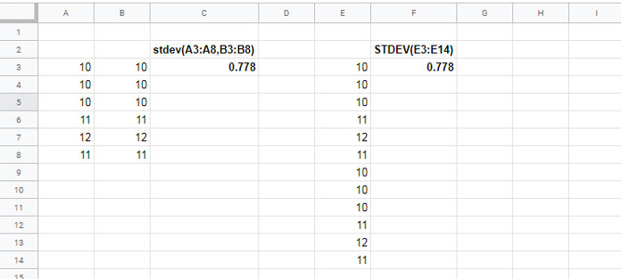
Both methods will return the same standard deviation if the values are the same.
You can also pass individual values like =STDEV(10, 15, 20).
Example 3: Conditional Standard Deviation Using FILTER
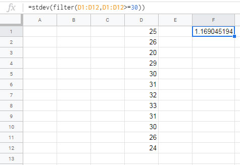
You can apply conditions before calculating standard deviation. For example, calculate the standard deviation of numbers greater than or equal to 30:
=STDEV(FILTER(D1:D12, D1:D12 >= 30))In this example, only values ≥30 will be considered. Text strings and blank cells are automatically ignored by STDEV.
Final Notes
- The STDEV function in Google Sheets ignores text and blanks.
- You can use STDEV.S interchangeably.
- Pair it with FILTER to apply conditions before calculation.


