")
")


")


")

")
")
 in Excel & Google Sheets")


In this tutorial, you’ll learn how to compare metrics like traffic or sales for a specific day — like today or yesterday — with the same day last week. And as a bonus, I’ll also show you how to compare the past 7 days of data with the 7 days before that, all in one go.
This kind of comparison is helpful in many real-world situations. Say you’re running a website and want to check how much traffic you got yesterday compared to the same day last week. That matters because traffic often varies by day — for example, weekends usually behave differently than weekdays. So it makes more sense to compare Sunday with last Sunday, not Monday.
The same logic applies to other metrics — sales, attendance, purchases, expenses, you name it.
Also, if you’re working with data that includes multiple entries per day (like several sales in a day), you’ll want to sum things up first before comparing.
I’ve kept all of that in mind while putting together this method to compare same day last week data in Google Sheets.
Compare a Specific Day (Today or Yesterday) With the Same Day Last Week
Let’s start with a simple example. You have:
- Column A: Dates
- Column B: The values you want to compare (sales, traffic, etc.)
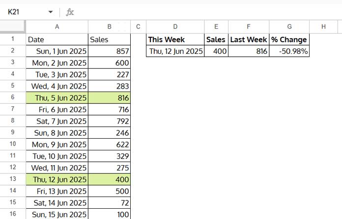
Step 1: Pick the date
In D2, enter the date you want to analyze — maybe today’s date or yesterday’s.
Example:
12/6/2025
Step 2: Get the value for that day
In E2, use:
=SUMIF(A2:A, D2, B2:B)Step 3: Get the value for the same day last week
In F2, use:
=SUMIF(A2:A, D2-7, B2:B)Step 4: Calculate the change
In G2, use:
=TO_PERCENT((E2 - F2) / F2)This gives you the percentage change. A positive value means this week’s number is higher than last week’s.
Compare the Last 7 Days With the Previous 7 Days
In this part, “this week” means the last 7 full days (excluding today). And “last week” is the 7 days before that. This way, you’re comparing two complete periods — no partial data.
Assume:
- Column A: Dates
- Column B: Sales (or whatever metric you’re tracking)
You can grab a copy of the sample sheet here.
Bonus: The sample sheet uses formulas to automatically generate rolling dates, so the data stays fresh on its own — no manual updates needed.
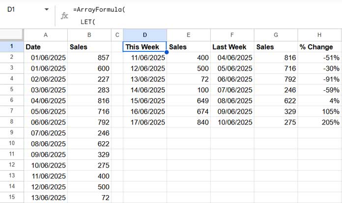
Paste this formula in D1:
=ArrayFormula(
  LET(
    header, HSTACK("This Week", "Sales", "Last Week", "Sales", "% Change"),
    thisweek, TO_DATE(SEQUENCE(7, 1, TODAY()-7, 1)),
    lastweek, TO_DATE(SEQUENCE(7, 1, TODAY()-14, 1)),
    thisweeksum, SUMIF(A2:A, thisweek, B2:B),
    lastweeksum, SUMIF(A2:A, lastweek, B2:B),
    change, TO_PERCENT((thisweeksum-lastweeksum)/lastweeksum),
    summary, HSTACK(thisweek, thisweeksum, lastweek, lastweeksum, change),
    VSTACK(header, summary)
  )
)
That’ll give you something like this:
What’s Going On in the Formula?
Let’s break down what each part of the formula is doing:
HSTACK(...)– This creates the five-column header: This Week, Sales, Last Week, Sales, and % Change.TO_DATE(SEQUENCE(7, 1, TODAY()-7, 1))– This generates the last 7 full days (excluding today) as proper dates, starting from 7 days ago to 1 day ago.TO_DATE(SEQUENCE(7, 1, TODAY()-14, 1))– This gives you the 7 days right before that, i.e., from 14 days ago to 8 days ago, also formatted as dates.SUMIF(A2:A, thisweek, B2:B)– Sums up the values in column B that match each of the 7 dates inthisweek.SUMIF(A2:A, lastweek, B2:B)– Same as above, but for the 7 dates inlastweek.TO_PERCENT((thisweeksum - lastweeksum) / lastweeksum)– Calculates the percentage change between this week’s and last week’s values.HSTACK(...)– Combines all five columns into a single table row: this week’s dates, this week’s totals, last week’s dates, last week’s totals, and the % change.VSTACK(header, summary)– Stacks the header row on top of the comparison table.
Together, this formula creates a quick, clean, and rolling “same day last week” comparison table — perfect for tracking sales, traffic, or any other time-based metric directly in Google Sheets.
Want a Chart Too?
You can create a bar or column chart from this 5-column table for a side-by-side comparison of same day this week vs same day last week.
Here’s how to do it:
- Update the headers in the formula for clearer chart legends:
- Replace
"Sales"(first occurrence) with"Sales This Week" - Replace
"Sales"(second occurrence) with"Sales Last Week"
- Replace
- Format the weekday labels:
- Select column D (this week’s dates)
- Go to Format > Number > Custom number format
- Enter
"ddd"to show abbreviated weekday names like Mon, Tue, etc.
- Hide column F (last week’s dates) to simplify the chart.
- Insert the chart:
- Select columns D to G
- Go to Insert > Chart
- Choose Bar chart or Column chart
This gives you a clean visual comparison of performance for the same weekdays across two weeks — ideal for reporting trends or spotting patterns.

Final Thoughts
This method makes it easy to compare today’s or yesterday’s data with the same day last week in Google Sheets. It also gives you the option to compare entire weeks in one go. Whether you’re analyzing traffic, sales, or any other daily metric, this technique helps you spot trends and make better decisions.
Related Resources
- Finding Week Start and End Dates in Google Sheets: Formulas
- Filter Data for a Specific Number of Past Weeks in Google Sheets
- Creating a Weekly Summary Report in Google Sheets
- How to Sum Values by the Current Week in Google Sheets
- Filter Data by Week (This, Last, or N Weeks Ago) – Google Sheets
- Filter or Find Current Week This Year and Last Year in Google Sheets
- How to Sum by Week of the Month in Google Sheets
Hi Prashanth,
Here’s a copy (removed by admin) where I have managed to use a query to display a pivot by month and year. Not sure how to make this work and display by day or week? So basically I’d like to show every day of the year if possible. If not then at least each week of the year if that is easier.
I have seen your Pivot report. The first column in the report is not month numbers. It’s “day of the year” grouping. So it’s not month and year as you have mentioned.
Hi Prashanth,
I’m a fan of all your google sheets tips.
I had a search of your archive and trying a few things myself, but one thing that is defeating me is finding a solution to this problem.
I want to list each day of the year by row and then in the columns, I’d like to show a sequence of years.
I’d then like to extract the sum of sales for each day of each year (my raw data shows the value of each sale and the date confirmed) so they are shown side-by-side allowing me to put together a chart or further analysis. Any tips much appreciated.
Andy
Hi, Andy H,
I think I can help you. You may require to use a Query formula. To help, I may require a mockup sheet. Consider sharing it (link/URL) in the comments below (I won’t publish it).