We can perform a Reverse VLOOKUP by virtually modifying the range using HSTACK or curly braces in Google Sheets. Of course, alternative solutions like INDEX-MATCH and the modern XLOOKUP function exist. Still, many users rely on VLOOKUP to find data to the left of a table. Do you know why?

Before we get into that, let’s understand what a Reverse VLOOKUP is and how to perform it.

What’s Reverse VLOOKUP in Google Sheets?

Reverse VLOOKUP refers to looking up data from right to left in a table. However, the VLOOKUP function is not designed for this by default.

In a regular VLOOKUP, the search key must be in the first column of your data range. For example, consider this formula:

=VLOOKUP(F3, B2:D5, 2, FALSE)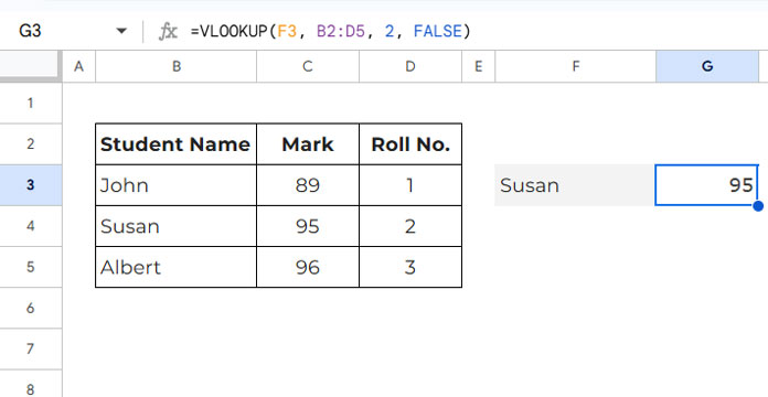

Here:

• The search key is “Susan” in cell F3.
• The range is B2:D5.
• The formula searches “Susan” in the first column of the range (B2:B5) and returns a value from the second column of the matching row.

Now, let’s look at a different scenario. How do you look up a roll number and return the corresponding student name or mark?

Reverse VLOOKUP addresses this problem effectively.

Reverse VLOOKUP in Google Sheets: How to Perform It

Scenario: Look up roll number 2 entered in cell F3 in the last column of the range B2:D5 and return the mark from the second column.

Here’s the formula:

=VLOOKUP(F3, {D2:D5, B2:C5}, 3, FALSE)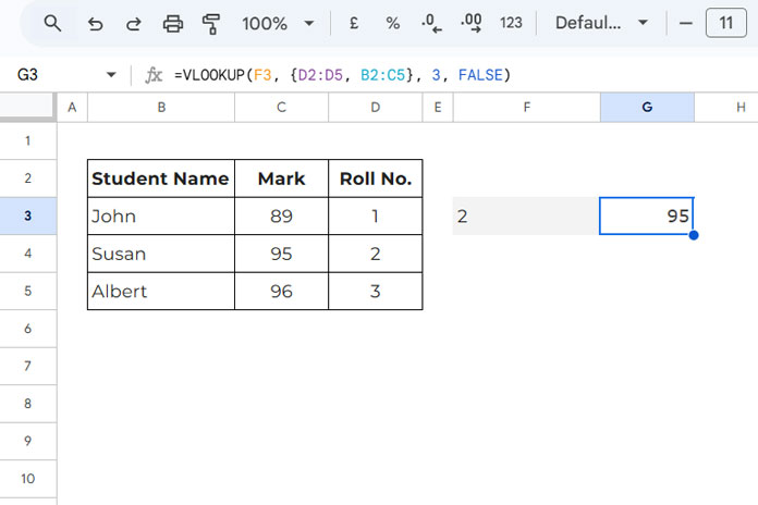

Since VLOOKUP cannot find data to the left, we modified the range virtually. The range is B2:D5, but we want to search in D2:D5. By rearranging the range with curly braces—{D2:D5, B2:C5}—we make D2:D5 the first column.

Now, the fields of the modified range are:

• Column 1: Roll No.
• Column 2: Student Name
• Column 3: Mark

Since the index is 3, the formula returns the mark of roll number 2 from the third column of this modified range.

Watch This Video to Master Reverse VLOOKUP in Google Sheets:

Returning Multiple Values

To return both the name and marks, use this formula:

=ArrayFormula(VLOOKUP(F3, {D2:D5, B2:C5}, {2, 3}, FALSE))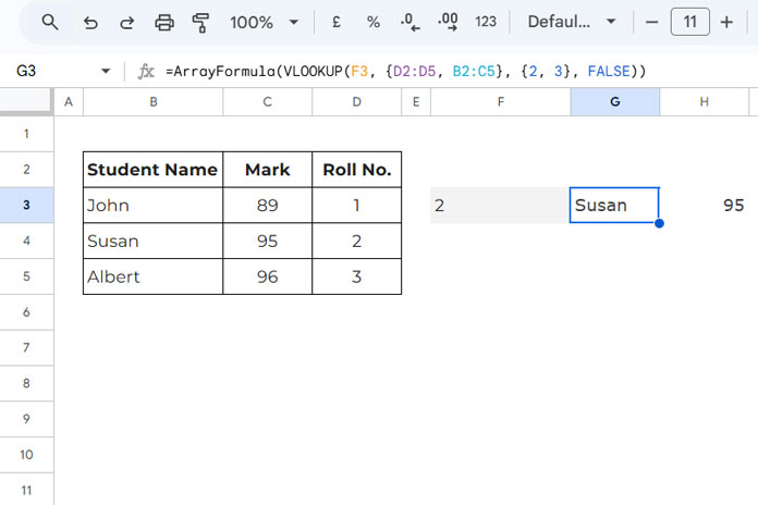

Tip: You can use HSTACK instead of curly braces to modify the range virtually. For example:

=ArrayFormula(VLOOKUP(F3, HSTACK(D2:D5, B2:C5), {2, 3}, FALSE))

Find Data Right to Left: Why Choose VLOOKUP over INDEX-MATCH or XLOOKUP?

One key benefit of using VLOOKUP over INDEX-MATCH or XLOOKUP for finding data to the left in Google Sheets is its ability to handle arrays.

Alternatives to Reverse VLOOKUP

Here are equivalent formulas:

• INDEX-MATCH:

=INDEX(B3:C5, MATCH(F3, D3:D5, FALSE))

MATCH finds the roll number’s position in D3:D5, and INDEX offsets the rows in B3:C5 accordingly.

• XLOOKUP:

=XLOOKUP(F3, D3:D5, B3:C5)

XLOOKUP searches F3 in D3:D5 and returns the corresponding row from B3:C5.

Why VLOOKUP Excels

If you want to look up two roll numbers (e.g., in F3:F4) and return names and marks for both, use this formula:

=ArrayFormula(VLOOKUP(F3:F4, {D2:D5, B2:C5}, {2, 3}, FALSE))

The alternatives won’t work directly in such cases, making VLOOKUP a better choice for handling multiple lookups simultaneously.

Resources

• Case-Sensitive Reverse VLOOKUP in Google Sheets
• How to Perform a Reverse HLOOKUP in Google Sheets
• VLOOKUP with Multiple Criteria in Google Sheets: The Proper Way
• Retrieve Multiple Values Using VLOOKUP in Google Sheets
• LOOKUP, VLOOKUP, and HLOOKUP: Key Differences in Google Sheets
• VLOOKUP Last Record in Each Group in Google Sheets
• How to Use VLOOKUP on Duplicates in Google Sheets
• Google Sheets – VLOOKUP Adjacent Cells
• VLOOKUP and XLOOKUP: Key Differences in Google Sheets