Using the RANK function in a range to find the rank of numbers returns duplicate ranks if any number is repeated. So how can you rank without duplicates in Google Sheets?
We can consider rank without duplicates from two perspectives. One approach only considers the first occurrence of values, while the other increments the rank of any duplicates by 1.
Scenario #1: Incrementing the Rank of Duplicates by 1
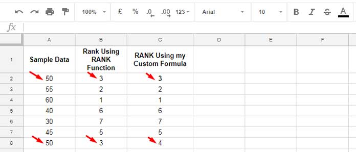
Please see the example screenshot below.

In cell B2, I have the regular RANK array formula, i.e., =ArrayFormula(IFNA(RANK(A2:A, A2:A, 0))), which returns the rank of the values in A2:A. I have another array formula in cell C2, which returns the rank without duplicates by incrementing the rank of duplicates by 1.
Since the number in cell A2 repeats twice (you can see that the number is the same in cell A8), the RANK formula in column B returns the same rank in cells B2 and B8.
However, the formula in column C intelligently returns unique ranks.
Formula and Explanation
Here is my formula in cell C2 that returns the rank without duplicates:
=ArrayFormula(LET(
   data, A2:A,
   seq, SEQUENCE(ROWS(data)),
   vZA, SORT(HSTACK(seq, data), 2, 0),
   seqvZA, HSTACK(seq, vZA),
   IF(NOT(A2:A), ,CHOOSECOLS(SORT(seqvZA, 2, 1), 1))
))
The above formula ranks the greatest value as rank #1. If you want the least value to rank #1, replace 0 (highlighted above) with 1.
Note: You can find another approach to solve this. Please check out my tutorial: How to Rank without Ties in Google Sheets.
Formula Breakdown:
Let’s start with the LET function, which we’ve used to assign names to the value expressions and then return the result of the formula expression.
LET(name1, value_expression1, [name2, …], [value_expression2, …], formula_expression)As per the formula:
name1:datavalue_expression1: A2:A
name2:seqvalue_expression2:SEQUENCE(ROWS(data))which returns the sequence numbers corresponding to the data to rank.
name3:vZAvalue_expression3:SORT(HSTACK(seq, data), 2, 0)
It first adds an array of sequence numbers with the rank range (the range to rank) and then sorts the rank range in descending order. The first column will be the sequence column, and the second column will be the data to rank.
name4:seqvZAvalue_expression4:HSTACK(seq, vZA)
Next, we again add the sequence numbers. So there will be three columns now: a sequence number column and the two-column sorted data from the previous step.
formula_expression:IF(NOT(A2:A), ,CHOOSECOLS(SORT(seqvZA, 2, 1), 1))
This sorts the three-column array from the previous step based on its second column in ascending order. Finally, we choose the first column, which contains the rank without duplicates.
The IF(NOT(A2:A), , ...) section ensures that the formula returns a rank only in non-empty cells so that you can use open data ranges.
Scenario #2: Rank Considering Only First Occurrences
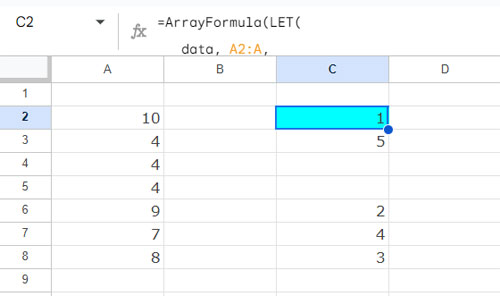
This is another method to rank without duplicates. Here we will consider only the first occurrences of the values in the range.
Formula:
=ArrayFormula(LET(
   data, A2:A,
   rc, COUNTIFS(data, data, ROW(data), "<="&ROW(data)),
   lt, IF(rc>1, , data),
   IFNA(RANK(lt, lt, 0))
))
To rank the least value as #1, replace 0 (highlighted in the formula) with 1.
Formula Explanation
It follows a very simple logic.
The following COUNTIFS formula returns the running count of the data:
COUNTIFS(data, data, ROW(data), "<="&ROW(data)) // named 'rc'The logical test checks whether the running count is greater than one. If true, it returns blank; otherwise, it returns the values:
IF(rc>1, , data) //named 'lt'Finally, the RANK function returns the ranks of the data without duplicates:
IFNA(RANK(lt, lt, 0)) //formula expressionResources
- Ranking a Non-Existing Number in Google Sheets Data
- How to Rank Group Wise in Google Sheets in Sorted or Unsorted Group
- Top 10 Ranking without Duplicate Names in Google Sheets
- Compare and Highlight Up and Down in Ranking in Google Sheets
- Find the Rank of an Item in Each Column in Google Sheets
- Highlight the Top 10 Ranks in Single or Each Column in Google Sheets
- How to Rank Data by Alphabetical Order in Google Sheets
- How to Rank Text Uniquely in Google Sheets


