By inputting the range of data points into a formula, we can promptly identify outliers in Google Sheets. The formula will return TRUE or FALSE Boolean values, indicating the presence of an outlier.
This eliminates the need for manual calculations, including determining quartile 1 and quartile 3, finding the interquartile range, and establishing lower and upper limit values for outlier identification. The formula handles all these tasks seamlessly.
Outliers:
In a given range, outliers are data points that significantly deviate from the majority of other data points.
Example:
Imagine you’re a steel distributor, and companies typically purchase materials ranging from 1 to 20 tons. Suddenly, an order for 100 tons arrives. This significant deviation raises eyebrows—Is it a typo, a genuine (but unusual) purchase, or something else?
Identifying outliers in data manually can be tedious. However, in Google Sheets, you can use an elegant formula to streamline the process. Simply input your data range, and the formula can flag potential outliers, often returning TRUE or FALSE values.
However, it’s crucial to note that blindly relying on TRUE/FALSE flags without considering context can lead to overlooking valid data.
Detecting Outliers in Google Sheets: Formula
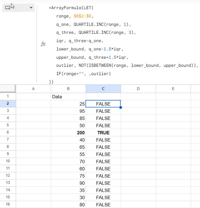
Here is the formula for swiftly identifying outliers in Google Sheets:
=ArrayFormula(LET(
   range, $B$2:$B,
   q_one, QUARTILE.INC(range, 1),
   q_three, QUARTILE.INC(range, 3),
   iqr, q_three-q_one,
   lower_bound, q_one-1.5*iqr,
   upper_bound, q_three+1.5*iqr,
   outlier, NOT(ISBETWEEN(range, lower_bound, upper_bound)),
   IF(range="", ,outlier)
))
Where:
- $B$2:$B is the range containing the data points for which you need to identify outliers. So, replace $B$2:$B with the actual data range.
I’ve used absolute references because we will use this formula for highlighting outliers in Google Sheets as well. We will explore that after the formula explanation below.
Formula Breakdown
The LET function in the outlier formula serves a key role in optimizing performance when identifying outliers in a large dataset by eliminating redundant calculations. Additionally, it allows us to assign names to ranges for clarity and simplicity.
For instance, in the formula above, we employ the LET function to calculate the Interquartile Range (IQR) and assign it the name ‘iqr.’ This named range is then used in subsequent calculations, avoiding the need for repetitive IQR calculations.
Furthermore, we name the data range $B$2:$B as ‘range,’ and wherever $B$2:$B appears later in the formula, we substitute it with ‘range.’ This approach streamlines the formula, making it more readable and easier to manage. Simply replace $B$2:$B with your desired data range, and the formula will unveil the outliers.
Syntax of the LET Function:
LET(name1, value_expression1, [name2, …], [value_expression2, …], formula_expression)How the Formula Finds Outliers in Google Sheets
Let me explain the outlier formula with the following table in Google Sheets:
| Names | Value Expressions | Remarks |
| range | $B$2:$B | |
| q_one | QUARTILE.INC(range, 1) | Represents the value below which 25% of data points fall when arranged in ascending (A to Z) order. |
| q_three | QUARTILE.INC(range, 3) | Represents the value below which 75% of data points fall when arranged in ascending (A to Z) order. |
| iqr | q_three-q_one | Represents the spread of the middle 50% of the data. |
| lower_bound | q_one-1.5*iqr | * Calculated value used to identify potential outliers below it. Typically calculated as Q1 – 1.5 * IQR. |
| upper_bound | q_three+1.5*iqr | * Upper boundary beyond which data points might be considered outliers. Calculated using Upper Limit = Q3 + 1.5 * IQR. |
| outlier | NOT(ISBETWEEN(range, lower_bound, upper_bound)) | The formula that finds outliers. The ISBETWEEN function returns TRUE if data points are between lower and upper limits. Wrapping the NOT converts FALSE to TRUE and TRUE to FALSE. |
| Formula Expression | IF(range=””, ,outlier) | Returns blank if data points in the range are blank, else returns the value determined by the outlier part of the formula. |
* 1.5 is a commonly used multiplier for defining the boundary.
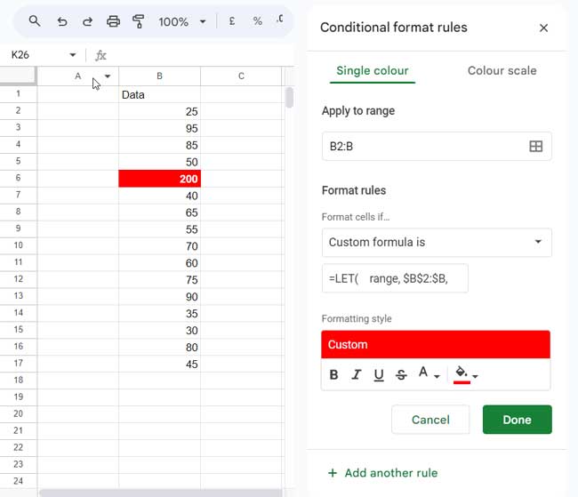
How to Highlight Outliers in Google Sheets
If you prefer highlighting data points rather than returning TRUE or FALSE to identify outliers, you can make a few adjustments to the formula. This will allow you to easily spot outliers in a dataset.
To highlight outliers without relying on any helper range, use the following custom rule in Conditional Formatting in Google Sheets:
=LET(
   range, $B$2:$B,
   q_one, QUARTILE.INC(range, 1),
   q_three, QUARTILE.INC(range, 3),
   iqr, q_three-q_one,
   lower_bound, q_one-1.5*iqr,
   upper_bound, q_three+1.5*iqr,
   outlier, NOT(ISBETWEEN(B2, lower_bound, upper_bound)),
   IF(B2="", ,outlier)
)
Replace $B$2:$B with your actual range and B2 with the cell ID where your range begins.
The changes in this highlight rule, compared to the formula that finds outliers, are minimal. In the outlier formula, we used the ‘range’ in ISBETWEEN and in the formula expression part.
In the custom formula rule, we used cell reference instead because we need to test each value (data points) individually, not as a range, for highlighting. Therefore, I removed the ARRAYFORMULA function since it is primarily used for expanding the ‘outlier’ and formula expression parts.
To apply the rule:
- Select the range.
- Click on Format > Conditional formatting.
- Under “Format rules,” choose “Custom formula is.”
- Enter the above formula (highlight rule).
- Click “Done.”
Conclusion
You can use either the formula or the highlighting rule to identify outliers in Google Sheets, and the choice is yours. I prefer the highlight rule.
If my dataset is very large, I would not directly resort to the highlight rule. Instead, I would first apply the formula that returns TRUE or FALSE and then use those values for highlighting. This approach improves performance.
In the above example, I would select B2:B, the data range, and use the following custom formula for highlighting:
=C2=TRUEResources:


