


")


")

")
")
 in Excel & Google Sheets")


Did you know you can use one FILTER function as the condition inside another FILTER in Google Sheets? It’s a neat trick — especially useful when you’re working with two connected tables or dependent datasets.
If the inner FILTER returns just one value, everything works smoothly. But if it returns multiple values, things get a little more interesting — and you’ll need a smarter formula to make it work.
Let’s break it down with a real example, covering both the easy case and the one where most people get stuck.
The Setup — Two Tables
Imagine you’re working with two related tables:
Table 1: Item & Quantity (A1:B)
| Item | Quantity |
|---|---|
| Raspberries | 10 |
| Blackberries | 10 |
| Pomegranate | 10 |
| Apple | 20 |
| Pineapple | 20 |
| Banana | 25 |
| Watermelon | 10 |
| Raspberries | 5 |
| Apple | 5 |
| Banana | 5 |
Table 2: Item & Unit Price (D1:E)
| Item | Unit Price |
|---|---|
| Raspberries | 3.00 |
| Blackberries | 3.00 |
| Pomegranate | 2.50 |
| Apple | 1.50 |
| Pineapple | 1.25 |
| Banana | 0.75 |
| Watermelon | 0.50 |
Your goal is to filter Table 1 based on a condition applied to Table 2 — for example, show only the items whose unit price is less than 2.
Case 1: When the Inner FILTER Returns One Item
Let’s start with the simpler scenario. Suppose you want to filter Table 1 to include only rows where the item’s unit price is less than 0.75.
Step 1: Use FILTER on Table 2
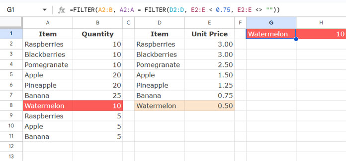
=FILTER(D2:D, E2:E < 0.75, E2:E <> "")This returns: "Watermelon"
Step 2: Plug That into Another FILTER on Table 1
=FILTER(A2:B, A2:A = FILTER(D2:D, E2:E < 0.75, E2:E <> ""))This works perfectly because the inner FILTER only returns one value — and A2:A = "Watermelon" is a valid condition across the range.
Case 2: When the Inner FILTER Returns Multiple Items
Now increase the threshold to less than 2, which returns multiple matches from Table 2.
Step 1: Update the FILTER on Table 2
=FILTER(D2:D, E2:E < 2, E2:E <> "")This returns: "Apple", "Pineapple", "Banana", and "Watermelon"
Step 2: Try That in Another FILTER (Will Fail)
=FILTER(A2:B, A2:A = FILTER(D2:D, E2:E < 2, E2:E <> ""))This formula fails with a #N/A error because you’re trying to compare a column (A2:A) with an array of multiple values — something FILTER doesn’t handle natively this way.
The Fix: Use XMATCH to Handle Multiple Values
Here’s the clean solution: use XMATCH to check whether each item from Table 1 appears in the filtered result from Table 2.
Working Formula:
=FILTER(A2:B, XMATCH(A2:A, FILTER(D2:D, E2:E < 2, E2:E <> "")))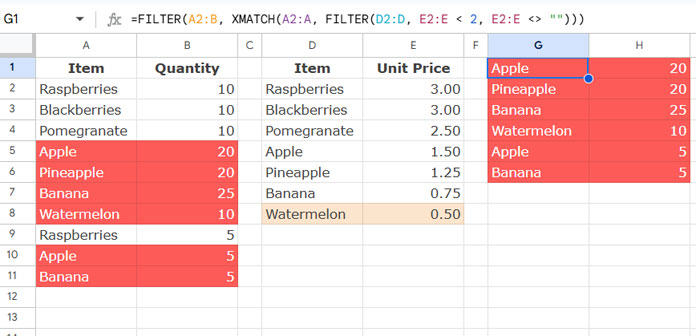
What This Formula Does:
FILTER(D2:D, E2:E < 2, E2:E <> "")pulls the items with a unit price under 2.XMATCH(A2:A, ...)checks whether each item in Table 1 appears in that list.- If there’s a match,
XMATCHreturns a number; otherwise, it returns#N/A. FILTERkeeps the rows whereXMATCHreturned a match (i.e., a number).
That’s how you can use one filter as the condition in another filter in Google Sheets, even when the inner filter gives multiple results.
Final Thoughts
When working with related tables — like a product list and its pricing — using one FILTER function as the condition inside another lets you build smart, responsive filters in Google Sheets.
Key Takeaways:
- For single-result filters, plug them directly into the outer condition.
- For multi-result filters, use XMATCH or REGEXMATCH to create a match-checking condition.
- This method works great for auto-updating lists, dashboards, and anything with dynamic filtering.
It’s a small trick — but it unlocks powerful logic, especially for more complex Google Sheets workflows.