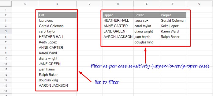
From a list, we can filter only uppercase, lowercase and proper case text string using a formula in Google Sheets. Yes! This tutorial is on Case Sensitive Filtering in Google Sheets.
I mean we can separate uppercase texts, lowercase texts and proper case texts from a list or table using three formulas of similar nature. If you feel this topic interesting, then please read on.
For case sensitive filtering we can use either the Exact function or the Regexmatch function with Filter function in Google Sheets. Also, we must use the Lower, Upper, Proper functions (as per requirement) as a combination with them.

Must Read: Google Doc Spreadsheet – Change Text to Upper, Lower and Sentence Case.
Both the Exact and Regexmatch can distinguish caps and small letters and return Boolean TRUE/FALSE accordingly. How?
The formulas under the following three titles will answer them
How to Test Whether a Text String Is Caps?
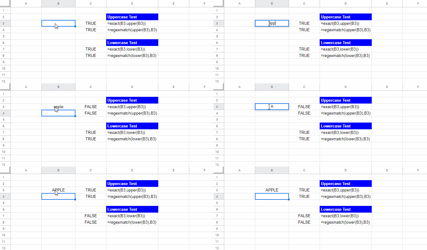
For example, cell B3 contains the string ‘apple’. To test whether the string is in capital letters (upper case), we can use the below formula.
EXACT Formula (to test whether a cell content is in capital letters):
=exact(B3,upper(B3))REGEXMATCH Formula (to test whether a cell content is in capital letters):
=regexmatch(upper(B3),B3)Both the above formulas will return TRUE if the cell content is in uppercase letters. Else, no doubt, the result would be FALSE.
I will explain how we can use either of these formulas in the Filter function to extract Uppercase Text String in Google Sheets.
I’ll probably go ahead with the latter one (Regexmatch). Before that see the similar (two each) Lowercase and Proper case formulas.
How to Test Whether a Text String Is Small?
Here we just need to replace the function UPPER with SMALL as below.
EXACT Formula to Test Lowercase String:
=exact(B3,lower(B3))REGEXMATCH Formula to Test Lowercase String:
=regexmatch(lower(B3),B3)
How to Test Whether a Text String Is Proper Case?
Similar to testing text string for small/upper letters only, we can use Proper function to test proper case text. Here also both the Exact and Regexmatch will come in use.
Formula to Test Proper Case Using Exact Function:
=exact(B3,PROPER(B3))Formula to Test Proper Case Using Regexmatch Function:
=regexmatch(PROPER(B3),B3)How to Filter Uppercase, Lowercase and Proper Case Text in Google Sheets
The question is how to use the above two (Exact and Regexmatch) formulas in a list. For that, we can use the Filter function.
In the above examples, we have used the Exact and Regexmatch functions with Upper, Small, and Proper functions to test a single text in cell B3. But when using these two functions to test a list (range), in standalone use, you must depend on the ArrayFormula function.
For example;
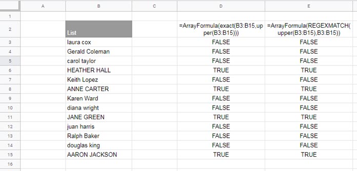
=ArrayFormula(exact(B3:B15,upper(B3:B15)))
=ArrayFormula(REGEXMATCH(upper(B3:B15),B3:B15))
Since we are going to use these two functions within Filter as the criteria we can avoid using the ArrayFormula function. This additional function is not required to populate an array when using Filter.
Just see the values in column D and E. Wherever the formulas return TRUE in column D and E, the corresponding row has names in capital letters in column B.
The logic lies in this Boolean TRUE to filter Uppercase, Lowercase and Proper Case Text in Google Sheets.
You need to filter the rows containing TRUE in order to filter uppercase names.
Formula to Filter Uppercase Text in Google Sheets:
=filter(B3:B15,exact(B3:B15,upper(B3:B15))=TRUE)Change Upper to Lower to filter lowercase names from the list.
Formula to Filter Lowercase Text in Google Sheets:
=filter(B3:B15,exact(B3:B15,LOWER(B3:B15))=TRUE)For filtering proper case strings, replace Lower with Proper.
Formula to Filter Proper Case Text in Google Sheets:
=filter(B3:B15,exact(B3:B15,PROPER(B3:B15))=TRUE)Case Sensitive Filter – Multiple Columns (Table)
As you can see, in all the examples above, there is only one column (list) to filter.
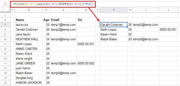
If you want to apply these filter formulas (Upper, Lower, and Proper) in the first column of a table (B3:E15 instead of B3:B15) change =filter(B3:B15, to =filter(B3:E15,.
The rest of the parts of the formulas are the same. I guess, the below screen capture is self-explanatory.

This way you can do case sensitive filtering in Google Sheets.
You May Like:


