In this tutorial, I will explain how to use the OFFSET function with the help of some examples in Google Sheets.

We can use the OFFSET function in Google Sheets to return a shifted range reference from a starting base cell, thereby creating dynamic ranges in formulas.

In certain scenarios, we can also use the QUERY function to offset rows. We will explore this later.

The syntax is straightforward. Here it is.

Syntax and Arguments

Syntax:

OFFSET(cell_reference, offset_rows, offset_columns, [height], [width])

Arguments:

• cell_reference – The starting point from which you want to base the offset.
• offset_rows – A positive integer (shift down) or negative integer (shift up) specifying the number of rows to shift by.
• offset_columns – A positive integer (shift right) or negative integer (shift left) specifying the number of columns to shift by.
• height – (Optional) The height, in number of rows, of the range to be returned starting at the offset target.
• width – (Optional) The width, in number of columns, of the range to be returned starting at the offset target.

Now let’s delve into a detailed understanding of the arguments in the OFFSET function.

How to Use the OFFSET Function in Google Sheets

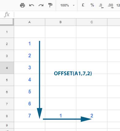
With the help of the following image and subsequent formula examples, I will demonstrate how to use the OFFSET function effectively.

Formula #1:

=OFFSET(A1, 7, 2)

Where:

• A1 is the cell_reference.
• 7 represents offset_rows.
• 2 represents offset_columns.

The above OFFSET formula refers to cell C8 and returns the value in this cell, similar to using the formula =C8.

Explanation:

1. Starting from cell A1, the formula shifts down seven rows due to the positive integer used in offset_rows, reaching cell A8.
2. It then shifts two columns to the right, also due to the positive integer used in offset_coumns, reaching cell C8.

While height and width elements are optional in most cases, they are crucial for creating dynamic ranges.

Formula #2:

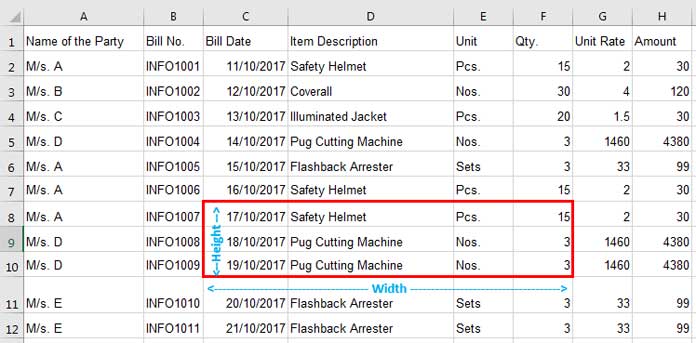
=OFFSET(A1, 7, 2, 3, 4)

In Formula #2, we’ve specified the height (3) and width (4), creating a range from cell C8 to F10.

I’ve marked the height and width on the image provided. The formula offsets 7 rows and 2 columns from cell A1, then returns a range of 3 rows and 4 columns starting from cell C8.

As mentioned earlier, we can utilize the QUERY function to some extent to achieve similar functionalities as the OFFSET function, particularly for offsetting rows.

=QUERY(A1:H, "Select C, D, E, F limit 3 offset 7", 0)

This QUERY will return the same range as described above.

Advanced Formula Examples

The OFFSET function introduces dynamism to ranges in Google Sheets. To grasp its utility, let’s explore the following examples.

Example 1: OFFSET Function with the SUM Function in Google Sheets

In the examples below, we replace the range reference in the SUM function with either the OFFSET or INDIRECT functions.

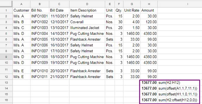
We’ve utilized four formulas in cells H13:H16 to sum the range H2:H12. Please refer to the image below.

The initial SUM formula in H13 is:

=SUM(H2:H12)

The alternative formula in H14 is:

=SUM(OFFSET(A1, 1, 7, 11, 1))

Here, the base to offset is cell A1. To obtain the shifted range reference H2:H12 from cell A1, we offset one row and seven columns (B to H). The height is 11 (rows), and the width is 1 (column), resulting in the OFFSET function within the SUM function referring to H2:H12.

In the formula in cell H15, where the base to offset is cell H1, no columns are shifted. Therefore, we specify the offset columns as 0 (zero):

=SUM(OFFSET(H1, 1, 0, 11, 1))

We can replace part of the range reference with an OFFSET formula on either side of a range. For instance, in the formula in cell H16:

=SUM(H2:OFFSET(H12, 0, 0))

Here, we replace H12 in the range H2:H12 with the OFFSET function.

As a side note, the INDEX and INDIRECT functions can achieve similar results:

Using INDEX:

=SUM(H2:INDEX(H12))

Using INDIRECT:

=SUM(H2:INDIRECT("H12"))

Example 2: Dynamic Ranges Using the OFFSET Function in Google Sheets

We can utilize the OFFSET function to ensure that a formula range in Google Sheets updates appropriately when inserting rows either immediately before or after the range reference. It’s important to note that the regular range will update accordingly when inserting rows within the range.

For instance, consider a SUM formula with a range reference of H2:H12. With the following formula, any new rows inserted at the beginning of the range, i.e., immediately above H2, will be included in the sum:

=SUM(OFFSET(H1, 1, 0):H12)

To create a fully dynamic formula, we can slightly modify it:

=SUM(OFFSET(H1, 1, 0):OFFSET(H13, -1, 0))

With this adjustment, we can insert rows both at the beginning (immediately above H2) and at the end (immediately after H12) of the sum range, ensuring the formula adapts dynamically.

Example 3: OFFSET Function with the SUBTOTAL Function in Google Sheets

The SUBTOTAL function typically returns an “Argument must be a range” error when any expression is used within the range. However, it does not encounter this issue when combined with the OFFSET function.

Here’s an example of how OFFSET and SUBTOTAL can be used together:

=SUBTOTAL(109, OFFSET(H1, 1, 0):OFFSET(H13, -1, 0))

This formula utilizes a dynamic range and calculates the total in the range H2:H12. Additionally, it excludes values in any hidden rows from the summation.

Resources

With the introduction of Lambda helper functions (LHFs), the utilization of the OFFSET function has increased. This is because we often employ REDUCE, one of the LHFs, for various advanced data manipulation techniques, supporting a single array.

However, when dealing with multiple arrays, we may find it necessary to utilize the OFFSET function. You can explore examples of this and other techniques in the tutorials below.

1. How to Offset Match Using Query in Google Sheets.
2. Vlookup and Offset Multiple Criteria in Google Sheets (Array Formula).
3. Search Value and Offset Cells in Google Sheets.
4. Auto-Expand Named Ranges in Google Sheets to Accommodate New Rows.
5. How to Use Dynamic Ranges in SUMIF Formula in Google Sheets.
6. XLOOKUP and Offset Results in Google Sheets
7. Consecutive Dates to Date Ranges in Google Sheets: The REDUCE Method
8. Conquer Duplicate IDs: Master Left, Right, Inner, & Full Joins in Google Sheets