How to Number Rows as 1, 1.1, 1.2, 1.3 in Google Sheets

If you want to number rows as 1, 1.1, 1.2, 1.3, 2, 2.1… in Google Sheets, you’re looking for a structured, outline-like approach to numbering. This can be achieved with a formula that lets you create sub-levels under each main row number. In this tutorial, we’ll show you how to set it up.

Setting Up Numbering Rows as 1, 1.1, 1.2, 1.3 in Google Sheets

This numbering style relies on defining two input columns. One column sets the main sequence (e.g., 1, 2, 3), and the other specifies each main number’s sub-levels. Here’s a step-by-step guide to create it in Google Sheets.

Hierarchical numbering of rows in Google Sheets, displaying sequences like 1, 1.1, 1.2, 1.3, and 2, 2.1, 2.2

Sample Input Values

Here’s an example of the input in columns A and B:

Main Sequence	Sub-Levels
1	5
2	3
3	4

With this input, you’ll generate a list like this:

1
1.1
1.2
1.3
1.4
1.5
2
2.1
2.2
2.3
3
3.1
3.2
3.3
3.4

Formula to Number Rows as 1, 1.1, 1.2, 1.3 in Google Sheets

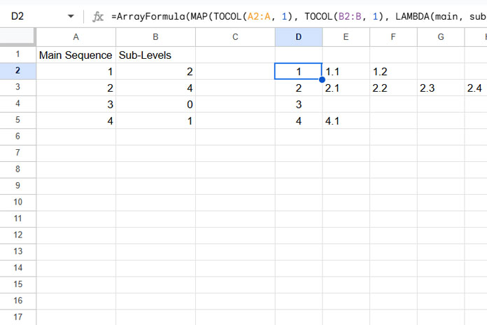
Once your main and sub-levels are set up in columns A and B, go to column C (starting in cell C2 or any empty cell) and paste this formula:

=ArrayFormula(
   TOCOL(
      MAP(TOCOL(A2:A, 1), TOCOL(B2:B, 1), 
         LAMBDA(main, sub, 
            TOROW(VSTACK(main, IF(sub>0, main&"."&SEQUENCE(sub),)))
         )
      ), 1
   )
)

This formula will number rows as 1, 1.1, 1.2, and so on in Google Sheets, adapting to your main sequence and sub-level entries.

Explanation of the Formula

Here’s how this formula works to number rows as 1, 1.1, 1.2, 1.3 in Google Sheets.

1. Creating the Sub-Sequence with SEQUENCE

The SEQUENCE function generates a series from 1 to the specified sub-level number in column B. For example, if cell B2 contains 5, then:

=SEQUENCE(B2)

This produces:

2. Combining the Main Sequence with Sub-Levels

Next, we combine column A’s main number with each sub-level SEQUENCE to create a 1.1, 1.2 style format. The formula for this is:

=ArrayFormula(IF(B2>0, A2 & "." & SEQUENCE(B2),))

For example, if A2 is “1” and B2 is “5”, this formula returns:

1.1
1.2
1.3
1.4
1.5

If B2 is 0, the formula returns a blank cell instead of generating any sub-level numbers.

3. Stacking the Main Number with the Sub-Sequence

To keep the main number as the top value followed by sub-levels, we use VSTACK:

=ArrayFormula(VSTACK(A2, IF(B2>0, A2 & "." & SEQUENCE(B2),)))

This will produce:

1
1.1
1.2
1.3
1.4
1.5

4. Ensuring a Single Row Format with TOROW

Using TOROW ensures that each hierarchical sequence is arranged in a single-row format (horizontally), as shown below:

=ArrayFormula(TOROW(VSTACK(A2, IF(B2>0, A2 & "." & SEQUENCE(B2),))))

5. Applying the Formula to Multiple Rows with LAMBDA and MAP

To number rows as 1, 1.1, 1.2, 1.3 for every row in columns A and B, we convert this logic into a LAMBDA function:

=LAMBDA(main, sub, ArrayFormula(TOROW(VSTACK(main, IF(sub>0, main & "." & SEQUENCE(sub),)))))

Here:

main is the main number from column A.
sub is the sub-level count from column B.

We use MAP to apply this LAMBDA function to all rows in columns A and B:

=ArrayFormula(MAP(TOCOL(A2:A, 1), TOCOL(B2:B, 1), LAMBDA(main, sub, TOROW(VSTACK(main, IF(sub>0, main & "." & SEQUENCE(sub),))))))

MAP applies the function to each main and sub-level entry in columns A and B.
TOCOL ensures the arrays from columns A and B are flattened, avoiding empty cells.

Applying the MAP function with LAMBDA to the main sequence and sub-levels in Google Sheets

The outer TOCOL in the original formula flattens this result range.

This approach allows you to automatically number rows as 1, 1.1, 1.2, 1.3 in Google Sheets, providing flexible control over each main and sub-level.

You can use this method to organize data in an outline-like format directly within Google Sheets.