


")


")

")
")
 in Excel & Google Sheets")


We can now hyperlink a substring or part of the text in a cell in Google Sheets. That means insert multiple hyperlinks within a cell in Google Sheets is now possible — a feature many users had been waiting for!
Earlier, when hyperlinking a (whole) text in a cell by clicking Insert > Link, Google Sheets would insert a HYPERLINK formula into the cell.
As you may know, formulas in Google Sheets start with an equal sign (=), and a cell can only contain one functioning formula. So there was no way to insert two separate, working formulas (and thus multiple hyperlinks) within a single cell.
In the past, this limitation meant that it wasn’t possible to insert multiple hyperlinks within a cell in Google Sheets. But now, things have changed slightly. Let me clarify.
Example: Insert Menu Link Option in Google Sheets
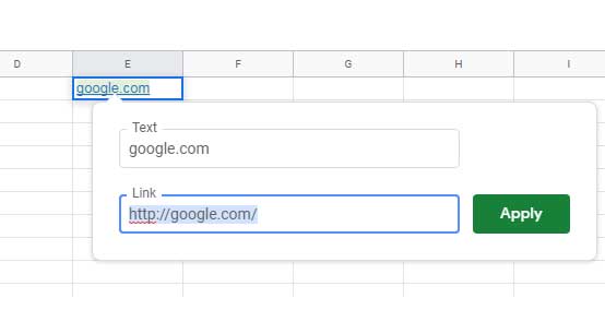
Say you insert a hyperlink in cell E1 by using the Insert > Link menu. The label (the visible blue text) is “Google,” and the URL is http://www.google.com/.
Now try entering the following formula in cell E2:
=FORMULATEXT(E1)Earlier, this would return the formula used to create the hyperlink:
=HYPERLINK("http://www.google.com/", "Google")You could also view this in the formula bar by selecting E1.
But now, if you insert a hyperlink using the same Insert > Link method, the link will still work — yet FORMULATEXT will return #N/A (invalid formula parse result). That’s because there’s no formula anymore, just a rich-text hyperlink directly embedded in the cell!
Two Ways to Insert Hyperlinks in Google Sheets (And Their Key Difference)
Today, there are two methods to insert hyperlinks in Google Sheets:
- Using the HYPERLINK function
- Using Insert > Link from the menu
These options existed earlier as well, but the result was the same — you could only insert one hyperlink per cell using either method.
Why? Because both methods used the HYPERLINK formula behind the scenes.
Formula Approach
To create a hyperlink using a formula, follow this syntax:
HYPERLINK(URL, [link_label])Example:
=HYPERLINK("https://google.com", "Google")I’m not going into more detail here — the example is self-explanatory.
Insert Menu Approach (Legacy)
This approach is best for inserting a single hyperlink — but hang tight, I’ll show you how to insert multiple hyperlinks within a cell in Google Sheets shortly.
When you type a domain name in a cell (like infoinspired.com in cell B2), Sheets may automatically hyperlink it.
If you want to link regular text (e.g., “infoinspired”), select the text, click Insert > Link, and enter the desired URL in the popup field (refer to screenshot #1).
Insert Multiple Hyperlinks within a Cell in Google Sheets – New Feature!
Now for the exciting part — here’s how to insert multiple hyperlinks within a cell in Google Sheets using the latest rich-text editing feature.
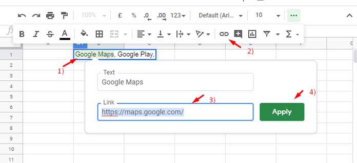
Let’s say cell B1 contains the comma-separated text: Google Maps, Google Play
Here’s how I’m adding two different hyperlinks to these words in the same cell.
- Double-click cell B1 or press
F2to edit. - Highlight “Google Maps” and press
Ctrl + K(Windows) or⌘ + K(Mac).
Alternatively, use the Insert link icon from the toolbar. - Type the link in the field and click Apply.
- Next, select “Google Play” and repeat the steps above.
That’s it!
How to Access the Links in the Cell
Wondering how to jump to those two web addresses?
There are two easy ways:
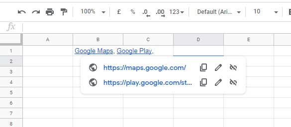
- Hover over cell B1 – a popup will show both hyperlinks.
- Double-click cell B1 – click either linked text to open the corresponding URL.
That’s all about how to insert multiple hyperlinks within a cell in Google Sheets. Thanks for reading — enjoy using this new feature in your Sheets workflow!
Resources
- Search for a Value and Hyperlink the Found Cell in Google Sheets
- Hyperlink to VLOOKUP Result in Google Sheets (Dynamic Link)
- Extract URLs from Hyperlinks in Google Sheets (No Scripting)
- UNIQUE Duplicate Hyperlinks in Google Sheets – Same Labels Different URLs
- How to Create a Hyperlink to an Email Address in Google Sheets
- Hyperlink Max and Min Values in Column or Row in Google Sheets
- Hyperlink to Index-Match Output in Google Sheets
- Hyperlink to Jump to Current Date Cell in Google Sheets
- Jump to the Last Cell with Data in a Column in Google Sheets (Hyperlink)
- Hyperlink Calendar Dates to Events in Google Sheets
- Using HYPERLINK with FILTER Function in Google Sheets
Okay, I did all this, but when I try to download it as a PDF, my links aren’t clickable. Help please!
That’s actually a limitation of Google Sheets’ PDF export. Unfortunately, it can’t be fixed with a formula or any standard setting in the sheet.