If you’re working with data where dates are spread across rows — like shipment records, project logs, or attendance sheets — you might want to quickly find the earliest date in each row.
Sounds simple enough, right? But there’s a catch: blank cells.
By default, Google Sheets doesn’t handle blanks the way you’d expect. Instead of leaving a row empty when there’s no data, you’ll often see a confusing 0 or a weird placeholder date like 30-Dec-99. That happens because Sheets is interpreting blanks as zero values and then formatting them as dates.
In this post, we’ll go through a few easy (and some advanced) ways to get the minimum date per row while ignoring blanks in Google Sheets. And if the entire row is empty? You’ll get a clean blank, just the way it should be.
Why Do Blanks Break the MIN Formula?
Here’s the issue in plain English:
- If at least one date exists in the row → MIN works fine.
- If the row is completely untouched → Sheets reads it as
0. - If a date was entered and later deleted → Sheets still remembers it, so you get
30-Dec-99(that’s “zero” formatted as a date).
This is why we can’t rely on plain MIN. We need a formula that ignores blanks properly.
Example Data
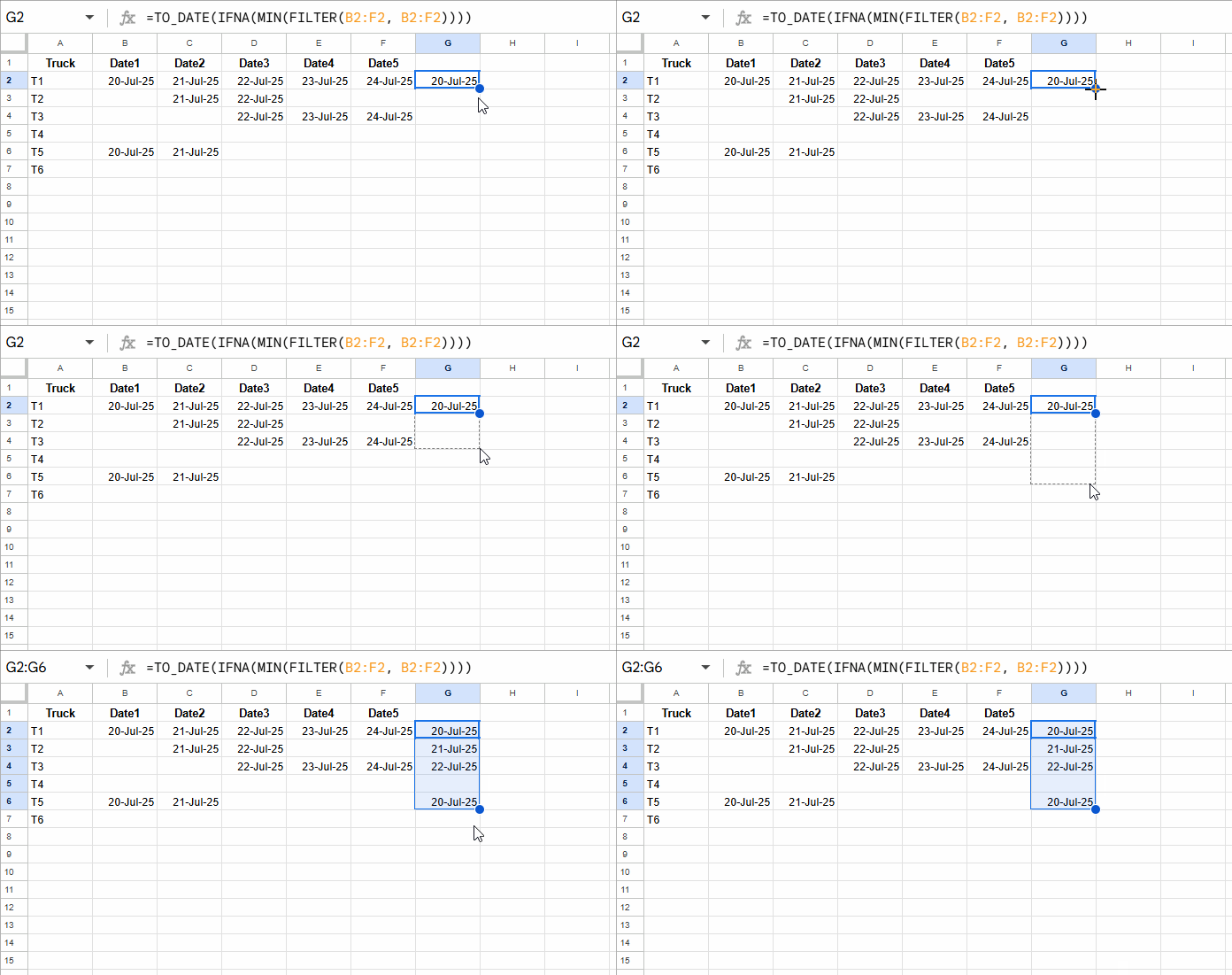
Suppose you have the following data in the range A1:F7:
| Truck | Date1 | Date2 | Date3 | Date4 | Date5 |
| T1 | 20-Jul-25 | 21-Jul-25 | 22-Jul-25 | 23-Jul-25 | 24-Jul-25 |
| T2 | 21-Jul-25 | 22-Jul-25 | |||
| T3 | 22-Jul-25 | 23-Jul-25 | 24-Jul-25 | ||
| T4 | |||||
| T5 | 20-Jul-25 | 21-Jul-25 | |||
| T6 |
Notice how some rows are fully populated, some partially, and some completely empty. We want the formula in column G to return the earliest shipment date per row, ignoring blanks — and if a row has no shipments, just stay blank.
Method 1: Simple Drag-Down Formula
The easiest solution is to use FILTER with MIN. Place this in G2 and drag it down:
=TO_DATE(IFNA(MIN(FILTER(B2:F2, B2:F2))))
How it works:
FILTER(B2:F2, B2:F2)→ removes blank cells.MIN(...)→ finds the earliest date left.IFNA(...)→ returns blank instead of#N/Afor empty rows.TO_DATE(...)→ ensures the result is shown as a date, not a serial number.
✅ Great for small datasets.
❌ Needs to be copied down manually.
Method 2: Array Formula with BYROW + LAMBDA
With a LAMBDA formula, you can easily get min date ignoring blanks in each row in Google Sheets. The result spills automatically, so there’s no need to drag formulas down.
=BYROW(B2:F, LAMBDA(row, TO_DATE(IFNA(MIN(FILTER(row, row))))))This applies the same calculation to each row in your range.
Why this method stands out:
- Spills automatically → no need to copy formulas down.
- Scales easily → new rows are handled automatically.
- Keeps your sheet clean → just one formula instead of many.
Method 3: The Old-School DMIN Hack
Before BYROW and LAMBDA existed, advanced users relied on DMIN. It’s clunky but still works:
=ArrayFormula(
   TO_DATE(
      IFERROR(1/DMIN(
         VSTACK("", TRANSPOSE(B2:F)),
         SEQUENCE(ROWS(B2:B)),
         VSTACK(IF(,,), IF(,,))
      )^-1)
   )
)
Here’s what’s happening:
TRANSPOSE(B2:F)→ flips rows into columns (because DMIN only works column-wise).VSTACK("", …)→ adds a fake header row, which DMIN needs.SEQUENCE(ROWS(B2:B))→ generates the correct column index for each row.1/x^-1→ forces an error on empty rows (instead of0).IFERROR+TO_DATE→ clean results, formatted as dates.
This method is more of a “formula hack” now. It’s fun to know, but for everyday work, stick to BYROW or the simple drag-down formula.
Conclusion
We’ve covered three reliable ways to get the min date ignoring blanks in each row in Google Sheets:
- Drag-down formula → quick and easy for smaller ranges.
- BYROW + LAMBDA → the cleanest, most modern option that updates automatically.
- DMIN hack → an older workaround, still useful for learning.
With these methods, you’ll always get the earliest valid date in each row—without running into errors, 0 values, or the confusing 30-Dec-99 placeholder.
Related Resources
- How to Exclude Zeros from MIN Function Results in Google Sheets
- Find Min or Max in a Google Sheets Matrix and Return Row Data
- Highlight Min Excluding Zeros and Blanks in Google Sheets
- Find the Column Header of the Min Value in Google Sheets
- Find and Filter the Min or Max Value in Groups in Google Sheets


