")
")


")


")

")
")
 in Excel & Google Sheets")


This post is all about how to find the MIN and MAX equivalent formulas for strings in Google Sheets.
Since MIN() and MAX() don’t work directly with text, we need alternatives. Luckily, we can use functions like QUERY, SORTN, or even a COUNTIF + XLOOKUP combo to return the max and min strings (alphabetical order) in Google Sheets.
I’ll walk you through all of them so you can pick the formula that suits your workflow best.
Example Data in Google Sheets
Here’s a small dataset of strings and their positions when sorted alphabetically (A–Z):
| Strings | Position (Alphabetical Order) |
|---|---|
| ACR | 0 |
| LMN | 1 |
| OPQ | 2 |
| PQR | 3 |
| WX315 | 4 |
| WX316 | 5 |
| WXYZ | 6 |
| WXYZ | 6 |
| WXYZ | 6 |
From this:
- The minimum string is
"ACR"(position 0). - The maximum string is
"WXYZ"(position 6).
How Alphabetical Order Works with Strings
If you sort the strings in ascending (A–Z) order, they’ll appear like this:
=SORT(A2:A10)→ ACR, LMN, OPQ, PQR, WX315…
If you sort in descending (Z–A):
=SORT(A2:A10, 1, 0)→ WXYZ, WXYZ, WXYZ, WX316…
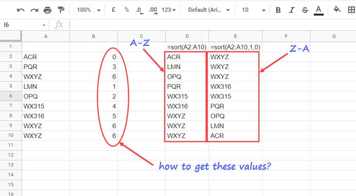
That’s exactly how Google Sheets decides which string is “min” and which is “max.”
Method 1 – COUNTIF + XLOOKUP Formula
One way is to calculate each string’s alphabetical position using COUNTIF.
In B2, enter:
=ArrayFormula(COUNTIF(A2:A10,"<"&A2:A10))Now we can use XLOOKUP to pull the actual max and min strings.
Max String:
=XLOOKUP(MAX(B2:B10), B2:B10, A2:A10)Min String:
=XLOOKUP(MIN(B2:B10), B2:B10, A2:A10)If you don’t want to use a helper column (B2:B10), you can replace it with the COUNTIF formula directly. The drawback is that COUNTIF will be recalculated multiple times, which is less efficient.
A better approach is to wrap it inside LET, so the array is calculated only once:
Max String (with LET):
=LET(ap, ARRAYFORMULA(COUNTIF(A2:A10, "<"&A2:A10)), XLOOKUP(MAX(ap), ap, A2:A10))Min String (with LET):
=LET(ap, ARRAYFORMULA(COUNTIF(A2:A10, "<"&A2:A10)), XLOOKUP(MIN(ap), ap, A2:A10))Method 2 – QUERY Function for Min and Max Text
The QUERY function in Google Sheets can return the max and min string directly without extra columns.
Max String:
=QUERY(A2:A10, "SELECT MAX(A) LABEL MAX(A)''")Min String:
=QUERY(A2:A10, "SELECT MIN(A) LABEL MIN(A)''")Simple and powerful—especially if you already use QUERY in your Sheets projects.
Method 3 – SORTN to Get the First and Last String (Recommended)
Here’s my go-to method.
In the beginning, I showed you how SORT can arrange strings alphabetically. But SORT alone can’t return just the first (min) or last (max) value. That’s where SORTN comes in—it sorts and also limits the output.
Max String:
=SORTN(A2:A10, 1, 0, 1, 0)Min String:
=SORTN(A2:A10)That’s it—clean and effective. Personally, this is the best formula for finding max and min strings in Google Sheets.
Wrap-Up: Finding Alphabetical Min/Max in Google Sheets
We’ve seen three different ways to find maximum and minimum strings in Google Sheets:
- COUNTIF + XLOOKUP – more manual, but flexible.
- QUERY – short and sweet.
- SORTN – the cleanest one-liner solution.
So, if you ever need the text equivalent of MIN() and MAX(), you now have a few solid options.
That’s all for today. Thanks for reading, and happy Sheet-ing!
Related Tutorials
- How to Exclude Zeros from MIN Function Results in Google Sheets
- Using MIN in Arrays in Google Sheets: A Complete Guide
- How to Sum, Avg, Count, Max, and Min in Google Sheets Query
- Find and Filter the Min or Max Value in Groups in Google Sheets
- Filter Max N Values in Google Sheets (Step-by-Step Guide)
Hi,
In my case, the correct “separated value” for the SORTN function was the semicolon, not the comma.
So
=SORTN(A2:A20;1;0;1;0)instead of
=SORTN(A2:A20,1,0,1,0)Hi, Saverio,
You are right. It’s because of the LOCALE settings. More info here – How to Change a Non-Regional Google Sheets Formula.
Hi Prashanth, I have sent you an email with the Sheet’s requirement for the analysis formula.
Hi, Ank,
I have responded via return mail. Please check your inbox.