To make the best use of PPMT function in Google Sheets, learn the other two financial functions – PMT and IPMT together with it.

For example, you can calculate the EMI of a loan using the PMT function. In that EMI, you can extract the interest component using the IPMT. Here the role of PPMT function is to extract the principal portion of the EMI.

In other words, you can bifurcate the principal and interest components of a monthly equated payment using IPMT and PPMT function respectively in Google Sheets. This is applicable to quarterly as well as yearly equal periodic payments.

That principal portion won’t be the same in the first period and subsequent periods. This rule is applicable to the interest portion too.

The charm of the above two financial functions are, you can use these to find the principal and interest components of any term during the loan tenure.

PPMT Function – Purpose and Syntax

The ‘P’ in the function PPMT stands for principal, that means PPMT denotes principal payment.

The purpose of the PPMT function in Google Sheets is to return the payment on the principal of an investment based on periodic, constant payments and a constant interest rate.

Syntax:

PPMT(rate, period, number_of_periods, present_value, [future_value, end_or_beginning])

Rate – It’s the annual interest rate.

Period – The amortization period. If Nper (see below) is 60, you can choose any number from 1 to 60 as the period.

Number of periods (Nper) – The total number of payments to be made (terms in months).

Present value (Pv) – The current value of the annuity (loan amount).

Future value (Fv) – Optional – The future value remaining after the final payment has been made.

End or beginning – optional – Whether payments are due at the end (zero) or beginning (one) of each period (zero by default).

Time to learn how to use the PPMT function in Google Sheets.

The Formula Examples to the PPMT Function in Google Sheets

Example:

Suppose you wish to buy a car to the tune of $20,000.00. Since you don’t have that much amount readily available, you decide to go for a car loan that with a tenure of 5 years.

Assume the interest rate per annum is 3.29%. Your estimated monthly payment (EMI) will be $362.00. You can calculate this EMI using the PMT function as below in Google Sheets.

=round(pmt(3.29%/12,60,20000))

I have just rounded the returned amount using the ROUND function. But that is not necessary though.

As mentioned, the annual interest is 3.29%. In the formula, that’s why I have divided it by 12 to make it monthly.

This payment includes both principal and interest payment. For calculating/extracting the interest payment, you can depend on the IPMT function in Google Sheets.

See my function guide to quickly learn the functions PMT, IPMT, and other important Google Sheets functions.

Using the PPMT function, you can extract the principal payment from this EMI. See the example below.

The PPMT Function in Monthly Periodic Payments

We have already the input values. See the above image. The only thing left for the PPMT (principal payment) calculation is the period of which you want to calculate the principal payment.

Let’s calculate the principal payment and interest payment for the first period (first loan repayment).

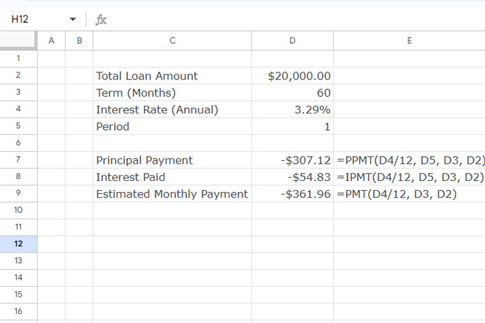
In cell D9 you can see the EMI that I have calculated using the PMT function as below.

=pmt(D4/12,D3,D2)

Result: $361.96

In cell D7 I have used the PPMT function to calculate the principal payment of the first period.

=ppmt(D4/12,1,D3,D2)

Result: $307.12

In compared to the PMT formula, there is only one additional parameter used in this PPMT formula, that’s the period.

Needless to say, the PMT amount will be the same for the whole tenure as it’s constant periodic payments. But the principal payment (PPMT) and interest payment (IPMT) will be different in each periodic payments.

With the help of PPMT and IPMT functions, we can find that amount.

Regarding the IPMT function, you just need to use the same PPMT formula and change the ‘P’ to ‘I’.

=IPMT(D4/12,1,D3,D2)

Result: $54.83

In concise;

PMT = IPMT + PPMT

In order to get the interest/principal component in the second, third or any other period of the loan repayment change the period in cell D5 accordingly.

Shorter the Tenure, Higher the EMI, But Lower the Interest [Example]

Now see this interesting calculation. I am going to change the loan tenure and see what happens.

If you opt a loan for a longer tenure, the EMI will be low. But the interest amount to be paid will be on the higher side.

The Use of PPMT Function in Google Sheets in Quarterly Periodic Payments

In case of quarterly repayment of a loan, the calculation of PPMT will be as follows.

• Convert the 3.29% of the annual interest rate to a quarterly rate, i.e.=3.29%/4.
• Convert the number of periods from months to quarters, i.e. =60/12*4.

Formula:

=ppmt(D4/4,D5,D3/12*4,D2)

How to Use The PPMT Function in Yearly Periodic Payments

In case of yearly repayment of a loan, the calculation of PPMT will be as follows.

• Use the 3.29% of the annual interest rate as it is.
• Convert the number of periods from months to years, i.e. =60/12.

Formula:

=ppmt(D4,D5,D3/12,D2)

Before winding up this tutorial one more thing. I have omitted two optional parameters in my example. They are;

future value (Fv):

The future value or balance of a loan after the final repayment will be 0. So you can omit that in formulas. If you want to keep any value, include that in the PPMT formula.

end_or_beginning:

Please see the Syntax portion above.