So, how do you calculate the modified internal rate of return in Google Sheets? Simple — use the MIRR function. In this post, I’ll walk you through how it works, where it differs from IRR, and how to set it up with your own data.
If you’ve read my earlier guide on the IRR function (you’ll find it under FINANCIAL FUNCTIONS in my function guide), this will feel like a natural extension. As the name hints, the M in MIRR stands for Modified. And yes, it modifies how we think about reinvestment returns.
MIRR vs. IRR — What’s the Difference?
Let’s quickly clear up the difference between these two functions.
- IRR assumes that all interim cash flows (i.e., profits you get each period) are reinvested at the same rate as the IRR — the return the project is expected to generate.
- MIRR lets you set two separate rates:
- One for the cost of investment (called the financing rate)
- One for the reinvestment return on future cash flows
In other words, the MIRR function in Google Sheets gives a more realistic picture by allowing different assumptions for borrowing costs and reinvestment returns. Handy, right?
MIRR Function Syntax
Here’s the syntax of the function:
MIRR(cashflow_amounts, financing_rate, reinvestment_return_rate)What each part means:
- cashflow_amounts – This is your list or range of cash flow values (like payments and returns). Make sure it includes at least one negative and one positive number.
- financing_rate – The interest rate you pay for the initial investment.
- reinvestment_return_rate – The interest rate you expect to earn from reinvesting the income you receive.
MIRR Formula Example in Google Sheets
Let’s make this hands-on.
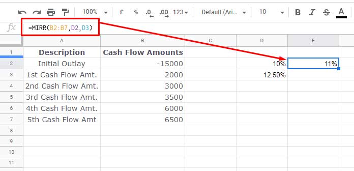
Here’s a small table — copy and paste it into the range A1:B7 of a new Google Sheet:
| Description | Cash Flow Amounts |
|---|---|
| Initial Outlay | -15000 |
| 1st Cash Flow Amount | 2000 |
| 2nd Cash Flow Amount | 3000 |
| 3rd Cash Flow Amount | 3500 |
| 4th Cash Flow Amount | 6000 |
| 5th Cash Flow Amount | 6500 |
Now let’s say:
- Your financing rate is 10% (or
0.1) - Your reinvestment return is 12.5% (or
0.125)
Here’s the formula you can use to calculate the MIRR:
=MIRR(B2:B7, 0.1, 0.125)Or if you prefer percentages:
=MIRR(B2:B7, 10%, 12.5%)This will return 11% as the modified internal rate of return.
Let’s tweak it a bit — change the reinvestment rate to 11%:
=MIRR(B2:B7, 0.1, 0.11)Now the result becomes 10%.
A Few Notes to Keep in Mind
- Your cash flows must occur at regular intervals (monthly, yearly, etc.), and in the correct order.
- You don’t need a range — you can also pass the cash flows directly as an array like this:
=MIRR(VSTACK(-15000, 2000, 3000, 3500, 6000, 6500), 10%, 12.5%)Or horizontally:
=MIRR(HSTACK(-15000, 2000, 3000, 3500, 6000, 6500), 10%, 12.5%)- If you forget to include a negative value (i.e., an investment outlay), Google Sheets will return a
#DIV/0!error — because MIRR can’t work without at least one payment.
Wrapping Up
So that’s how the MIRR function in Google Sheets works! It’s a great alternative to IRR when you want more control over your assumptions — especially if the reinvestment rate is different from your financing rate.
Try plugging in your own numbers to see how changes in those two rates affect your result. It’s a small formula, but super useful in real-world financial analysis.
Thanks for reading — and as always, feel free to explore more below if you’re on a spreadsheet deep dive.


