The IRR function in Google Sheets is a useful tool for estimating the return on an investment based on periodic cash flows.
In this post, I’ll walk you through how the IRR function works in Google Sheets, using a simple example.
What Is Internal Rate of Return (IRR)?
The internal rate of return (IRR) is the rate at which the net present value (NPV) of an investment becomes zero. In other words, it’s the interest rate that makes the present value of all future cash flows (inflows and outflows) equal to the original investment.
So if you’re investing in a project or startup and want to know how profitable it might be, IRR gives you a single percentage you can use to compare different opportunities. The higher the IRR, the more attractive the investment.
Why does NPV become zero when using IRR as the discount rate?
Because IRR is the rate at which the present value of future cash inflows exactly offsets the initial investment. When you plug the IRR into the NPV formula as the discount rate, you’re essentially asking, “How much is this investment worth today if I expect this exact return?” The answer is zero—because the return already equals the cost.
Things to Know Before Using IRR in Google Sheets
- The cash flows must be periodic—for example, monthly, quarterly, or yearly.
- The cash flow amounts don’t need to be equal; only the timing matters.
- The range should include at least one negative and one positive value to compute the IRR.
IRR Function Syntax in Google Sheets
IRR(cashflow_amounts, [rate_guess])Arguments:
- cashflow_amounts – A range or array of numeric values representing payments and income related to the investment. The first value is usually the initial investment (a negative number), followed by positive or negative future cash flows.
- rate_guess (optional) – An estimated IRR to help the function start its internal calculation. If omitted, Google Sheets uses 10% (0.1) by default. In most cases, you don’t need to provide this.
IRR Function Example in Google Sheets
Let’s say Project A requires an initial investment of $7,000, followed by these expected annual returns:
| Period | Cash Flow | Description |
|---|---|---|
| 0 | -7000 | Initial cost of the project |
| 1 | 2500 | Net income for Year 1 |
| 2 | 4500 | Net income for Year 2 |
| 3 | 1000 | Net income for Year 3 |
| 4 | 3800 | Net income for Year 4 |
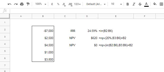
These cash flow values go into cells B2:B6. Here’s how you can calculate the internal rate of return using the IRR function in Google Sheets:
Formula:
=IRR(B2:B6)Result: 24.59%
That means over a period of four years, this project is expected to generate a return of around 24.59% per year.
IRR as a Discount Rate in NPV
To see why IRR is meaningful, let’s run a quick NPV calculation with a 20% discount rate:
=NPV(20%, B3:B6) + B2Result: $619.60 – This is the net present value of the investment when discounted at 20%.
Now, replace 20% with the actual IRR:
=NPV(IRR(B2:B6), B3:B6) + B2Result: 0
That confirms the definition—IRR is the rate that brings NPV to zero. This can help you compare the internal return of different projects, especially when deciding whether a return is good relative to your expected rate or cost of capital.
Wrapping Up
The IRR function in Google Sheets is a valuable tool for evaluating whether a project is worth pursuing. It gives you a clear idea of the return rate over time, especially when cash flows vary from period to period. You can also combine it with other functions like NPV to double-check your assumptions.
Thanks for reading! Hope this helped you understand not just the formula, but the logic behind it.


