There are three financial functions in Google Sheets for calculating the internal rate of return for a schedule of cash flows: IRR, XIRR, and MIRR. In this post, let me shed some light on how to use the XIRR function in Google Sheets.
We can use the XIRR function to calculate the internal rate of return of cash flows that are not periodic—in other words, not spaced at equal intervals.
The XIRR calculation excludes external factors like inflation, cost of capital, or various financial risks. That’s why it’s called the internal rate of return.
You can use either Excel or Google Sheets for the XIRR calculation. Here, I’m using Google Sheets for the explanation.
XIRR Function – Syntax and Arguments Explained
XIRR is a measure—or more precisely, an estimate—of an investment’s return when cash flows occur at irregular intervals. Let’s go over the syntax and arguments of this function, followed by an example.
Syntax
XIRR(cashflow_amounts, cashflow_dates, [rate_guess])In Excel, you might see the syntax as:
XIRR(values, dates, [guess])In our case:
values=cashflow_amountsdates=cashflow_datesguess=rate_guess
Arguments
- cashflow_amounts – A range or array containing a series of cash flows (income or payments) associated with the investment.
This array must include at least one negative and one positive cash flow for XIRR to return a result. - cashflow_dates – A range or array of dates corresponding to each cash flow.
- rate_guess – An optional estimate close to the expected result.
You can skip this. If omitted, Google Sheets uses a default guess of 0.1 (or 10%).
Example: Using the XIRR Function in Google Sheets
Let’s see how to use the XIRR function in Google Sheets to calculate the internal rate of return from a set of irregularly spaced cash flows. If your cash flows occur at regular intervals (like monthly or annually), consider using the IRR function instead.
Want to learn more about financial formulas in general? Check out my complete Google Sheets function guide.
Sample Data:
| Description | Cash Flow Amounts | Cash Flow Dates |
|---|---|---|
| Initial Outlay | -15000 | 01-Jan-2020 |
| 1st Cash Flow Amt. | 2000 | 01-Feb-2020 |
| 2nd Cash Flow Amt. | 3000 | 01-May-2020 |
| 3rd Cash Flow Amt. | 3500 | 01-Aug-2020 |
| 4th Cash Flow Amt. | 3500 | 01-Nov-2020 |
| 5th Cash Flow Amt. | 4000 | 01-Feb-2021 |
Assume the above data is in the range A1:C7, with the cash flow amounts in column B and the corresponding dates in column C.
As you can see, the dates are irregular. So, to calculate the internal rate of return, use the XIRR formula like this:
=XIRR(B2:B7, C2:C7)This will return 0.10, or 10%.
To display the result as a percentage, wrap it with the TO_PERCENT function:
=TO_PERCENT(XIRR(B2:B7, C2:C7))XIRR in XNPV
Let’s take it a step further. Suppose you want to calculate the net present value (XNPV) of the same investment using a discount rate of 10%.
In that case, the XNPV would return 0, because:
When the discount rate in XNPV equals the internal rate of return (XIRR), the net present value is zero.
Syntax:
XNPV(discount_rate, cashflow_amounts, cashflow_dates)Formula:
=XNPV(XIRR(B2:B7, C2:C7), B2:B7, C2:C7)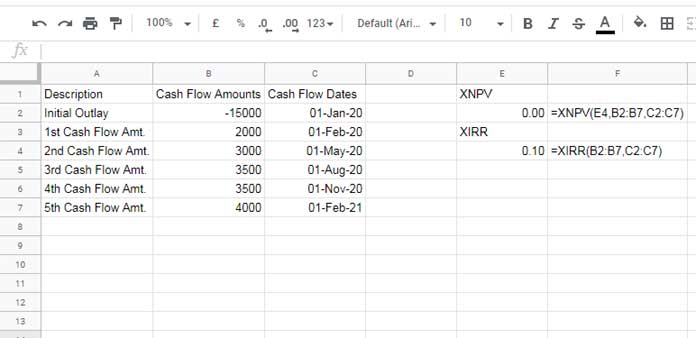
XIRR Function in Google Sheets – Summary
The XIRR function in Google Sheets is useful when your cash flows don’t follow a regular schedule. It provides a more accurate internal rate of return than the IRR function when dealing with irregular timing.
Just ensure:
- You include at least one negative and one positive cash flow.
- The dates are valid.
That’s all. Enjoy exploring your investment metrics!
FAQs
Q: What’s the difference between IRR and XIRR in Google Sheets?
A: IRR is used when cash flows occur at regular intervals, while XIRR handles irregular or non-periodic cash flow dates.
Q: What does it mean when XIRR returns a #NUM! error?
A: This usually means the input doesn’t include at least one negative and one positive cash flow, which is required for the XIRR calculation. Another possible reason is that the function couldn’t find a result that satisfies the internal rate of return after multiple iterations.
Q: Can I use XIRR without specifying the guess argument?
A: Yes. The guess is optional in Google Sheets. If omitted, it defaults to 10% (0.1).


