In this Google Sheets tutorial, we will create a formula to check if an entered date already exists and, if it does, generate the next available date. Additionally, you have the option to exclude weekends if desired.

To generate the next available date, we will utilize the WORKDAY.INTL function with XMATCH, IF, and ISNA functions in Google Sheets.

How can generating the next available date be beneficial?

Let me clarify how this works. The formula will check if the given date already exists in a list. If the date is already present, the formula will provide the next available date; otherwise, it will return the entered date.

This feature can be valuable in various scenarios, such as project scheduling, booking rooms, events, and many other instances where booked dates are spread out.

For instance, if the booked dates are 01 Jan 2023, 04 Jan 2023, 03 Jan 2023, 05 Jan 2023, and 07 Jan 2023, and another booking request is made for 04 Jan 2023, the formula will suggest 06 Jan 2023 as the next available date.

You can then enter the returned date in the list, avoiding duplicated date entries in a date column.

As mentioned, you can exclude weekends when generating the next available date.

Next Available Date Generator Formula for Google Sheets

Here is the formula to check if an input date already exists and, if it does, return the next available date; otherwise, return the entered date.

=IF(ISNA(XMATCH(C2,A:A)), C2, WORKDAY.INTL(C2, 1, "0000000", A1:A))

I’ve coded this formula assuming that the date you want to test is in cell C2, and the list of dates is located in column A.

This formula does not account for skipping weekends when generating the next available date. We’ll address such a formula next. Before that, let me explain the structure of this formula:

Anatomy of the Formula

We can break the formula down into three parts: XMATCH, WORKDAY.INTL, and the IF logical test.

Part #1: XMATCH

The XMATCH function, written as XMATCH(C2, A:A) in the formula, checks whether the input date in cell C2 already exists in the list of dates in column A.

Syntax:

XMATCH(search_key, lookup_range, [match_mode], [search_mode])

In this formula, C2 is used as the search_key, and column A:A is the lookup_range.

If the date is found, XMATCH will return the position where the date is located; otherwise, it will return #N/A.

We’ve enclosed the XMATCH formula with ISNA to return TRUE if the search returns #N/A and FALSE if it finds a match.

Part #2: WORKDAY.INTL

The role of the WORKDAY.INTL function is to generate the next available date. It is written as WORKDAY.INTL(C2, 1, "0000000", A1:A) in the formula.

Syntax:

WORKDAY.INTL(start_date, num_days, [weekend], [holidays])

Where:

• C2: This is the starting date (the date in cell C2).
• 1: This value represents the number of workdays to add. In this case, it’s set to 1, which ensures the next working day is calculated.
• "0000000": The text string to specifies weekends. In this case, "0000000" means that no days (0) are treated as weekends.
• A1:A: The range A1:A is used to identify holidays or non-working days. The formula excludes these dates when generating the next working day.

Part #3: IF

The IF function is used to determine whether the input date already exists and return the next available date accordingly.

Syntax:

IF(logical_expression, value_if_true, value_if_false)

The logical_expression is the output of the ISNA. If it evaluates to TRUE, the formula will return the date in C2. If it’s FALSE, the formula proceeds to the WORKDAY.INTL part (#3) to return the next available date.

In summary, if the input date in cell C2 is not found in the list (column A), it returns the same date. If the input date is already in the list, it calculates the next working day as the next available date.

That’s the logic behind our next available date generator in Google Sheets.

How to Generate the Next Available Date, Excluding Weekends

If you wish to exclude specific dates, such as weekends, when generating the next available date, you can modify the “0000000” part of the formula as follows:

In the above, the 7 zeroes indicate 7 workdays, where the first 0 represents Monday, and the last 0 represents Sunday. To exclude weekends, replace “0000000” with “0000011.” This adjustment ensures that Saturdays and Sundays are not considered as workdays when determining the next available date.

In short, a zero means that the day is a work day, and a 1 means that the day is a weekend.

Here is the formula to generate the next available date excluding Saturday/Sunday weekends.

=IF(ISNA(XMATCH(C2, A:A)), C2, WORKDAY.INTL(C2, 1, "0000011", A1:A))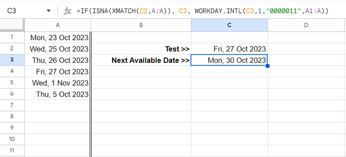

Generate the Next Available Date Based on a Condition in Google Sheets

Sometimes, you may need to generate the next available date based on a specific condition.

For instance, if you have hotel room numbers in column A and booked dates in column B, and you want to find the next available date for room #206, you would apply a condition.

The following formula returns the next available date for room #206:

=IF(ISNA(XMATCH(D2, FILTER(B:B, A:A=D3)), D2, WORKDAY.INTL(D2, 1, "0000000", B1:B))

This formula differs from our earlier formula in one aspect, specifically within the XMATCH.

In our previous next available date generating formulas, the lookup_range in XMATCH was simply A:A (date column). However, in this formula, it is FILTER(B:B, A:A=D3).

The FILTER function filters only the dates in B:B that match room #206 (D3) in A:A.

Syntax:

FILTER(range, condition1, [condition2, …])

Next Available Date Generator Template

Click the link below to preview and copy the Next Available Date Generator template for free:

NADG Template

The template contains three sheets:

1. NAD: Next Available Date
2. NAD_EW: Next Available Date (Excluding Weekends)
3. C_NAD: Conditional Next Available Date (Excluding Weekends)

You can use the templates in two ways:

1. With an existing list of dates: Copy and paste the dates into column A in the first two sheets and column B in the third sheet.
   • You only need to use one Sheet.
   • The locale setting of the template is “UK”. Open the copied template and click File > Settings to change the locale before you start using it.
2. Fresh: Empty the dates in column A in the first two sheets and column B in the last sheet. Enter the first date in cell A1 or B1, depending on which sheet you use.

Input your date to test in cell C2 in the first two sheets and cell D2 in the third sheet. The criterion goes to cell D3.

To change weekends, follow the relevant portion in the tutorial above.