How to Flatten Every Other Column in Google Sheets

Flattening every other column in Google Sheets means merging values from alternating columns into a single column. For example, you can consolidate data from columns A, C, and E into one column and columns B, D, and F into another. This can be useful for summarizing data using QUERY or performing lookups efficiently.

Fortunately, flattening every other column in Google Sheets is straightforward.

You can use curly brackets {} to combine alternating columns horizontally or apply the HSTACK function before flattening them.

Flattening Every Other Column in Google Sheets (Non-Dynamic)

Here’s an example:

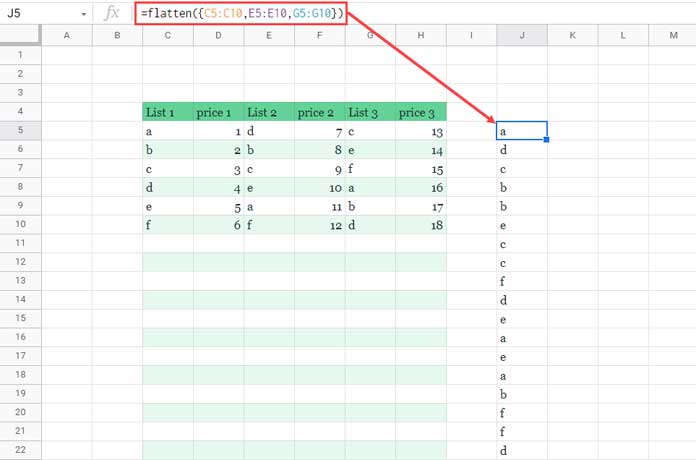
Example of flattening alternate columns in Google Sheets — image # 1

=FLATTEN({C5:C10,E5:E10,G5:G10})

=FLATTEN(HSTACK(C5:C10,E5:E10,G5:G10))

The above formulas flatten the ranges C5:C10, E5:E10, and G5:G10 into a single column.

Limitation of This Approach

Using curly brackets {} is only practical when dealing with a few columns. However, this method offers flexibility when flattening non-sequential columns.

Flexible Formula to Flatten Every Other Column in Google Sheets

Now, let’s create a more dynamic formula.

Steps:

Identify the column number of the first column in the range using:
=COLUMN(C4)
If the result is odd, use the ISODD function within FILTER; otherwise, use ISEVEN.
Apply the following formula to dynamically flatten every other column:

=FLATTEN(FILTER(C5:H10, ISODD(COLUMN(C4:H4))))

This formula filters C5:H10 based on whether the corresponding column number in C4:H4 is odd. The filtered columns are then flattened into a single column.

For a larger dataset, simply extend the range:

=FLATTEN(FILTER(C5:Z10, ISODD(COLUMN(C4:Z4))))

To flatten even-numbered columns instead, replace ISODD with ISEVEN.

Troubleshooting: Handling Blank Rows and Columns

1) Removing Blank Columns from the Flattened Output

If your range contains empty columns, they will create blank rows in the result. To exclude such columns, add a LEN check:

=FLATTEN(FILTER(C5:Z10, ISODD(COLUMN(C4:Z4)), LEN(C4:Z4)))

Here, LEN(C4:Z4) ensures only columns with headers (non-empty cells) are included.

2) Removing Blank Rows from the Flattened Output

If blank rows appear in the result, modify the formula by wrapping it in QUERY:

=QUERY(FLATTEN(FILTER(C5:Z, ISODD(COLUMN(C4:Z4)), LEN(C4:Z4))), "SELECT * WHERE Col1 IS NOT NULL")

3) Flattening Even-Numbered Columns

To flatten only even-numbered columns, modify the formula as follows:

=QUERY(FLATTEN(FILTER(C5:Z, ISEVEN(COLUMN(C4:Z4)), LEN(C4:Z4))), "SELECT * WHERE Col1 IS NOT NULL")

Flattening Both Odd and Even Columns in a Single Formula

Instead of using two separate formulas for odd and even columns, you can combine them into one:

=QUERY(
   {FLATTEN(FILTER(C5:Z, ISODD(COLUMN(C4:Z4)), LEN(C4:Z4))), 
     FLATTEN(FILTER(C5:Z, ISEVEN(COLUMN(C4:Z4)), LEN(C4:Z4)))}, 
   "SELECT * WHERE Col1 IS NOT NULL"
)

Note:

When using this formula, ensure that the number of columns in both flattened arrays is equal. If the first flattened set consists of five columns, the second must also have five columns. This mismatch can occur if some columns are missing headers, which may cause errors in the output.