In Google Sheets, we can group a date field using a Pivot Table in various ways, such as by Date, Month, Quarter, Year, and Year-Month. This tutorial explores the utilization of the GETPIVOTDATA function with these grouped dates in Google Sheets.
Throughout this tutorial, I will guide you through four examples. Specifically, we will create four distinct Pivot Tables from a single source dataset and employ the GETPIVOTDATA function to retrieve the necessary aggregated values.
Unfortunately, many users encounter challenges in decoding this process, often stumbling upon #REF! formula errors due to blindly adhering to the function’s syntax. Let’s unravel these common pitfalls:
- Original Column Mismatches: The
original_columnargument ideally should reflect the exact column name from the source dataset. However, ‘Pivot date grouping’ can introduce subtle modifications within the Pivot Table, leading to potential confusion. - Date Criterion Formatting: Whether a date has undergone ‘Pivot date grouping’ or not, it’s crucial to specify it as text within the pivot_item argument.
Let’s delve into the correct way to utilize the GETPIVOTDATA function with grouped dates in Google Sheets.
Sample Data and Pivot Table
Consider the following fictitious sample data with three columns.
| Country | Date of Travel | Number of Travelers |
| FR | 01/01/2023 | 5 |
| FR | 25/01/2023 | 15 |
| FR | 01/02/2023 | 10 |
| IT | 01/01/2023 | 6 |
| IT | 20/01/2023 | 8 |
| IT | 01/02/2023 | 10 |
Assume the above sample data is located in cell range A1:C7 in “Sheet1.” We are creating the Pivot Table in the same sheet starting from cell A9. Here are the steps to follow:
- Move to cell A9.
- Click on “Insert” > “Pivot Table.”
- In the “Data range” field, enter the correct range A1:C7.
- Select “Existing sheet” and enter A9 in the provided field.
- Click “Create” to insert the Pivot Table and open the sidebar Pivot Table editor panel.
- Drag and drop the field “Date of Travel” below
Rows. - Drag and drop the field “Country” under
Columns. - Under
Values, drag and drop the field “Number of Travelers” and ensure that “Summarize by” is set to SUM.
To access sample Sheets, Pivot Tables, and formulas, please click the button below and follow the on-screen instructions.
Using GETPIVOTDATA with Grouped Dates in Rows in Google Sheets
We have a Pivot Table report in Google Sheets that currently groups dates in Rows. How do we use the GETPIVOTDATA function with these grouped dates in Rows?
In the first example, we will not employ manual date grouping, meaning no Month, Year, Quarter, etc. grouping.
Example 1 (Filter by Rows)
(Refer to Sheet1 in the Sample Sheet above)
The following formula retrieves the total number of travelers on 01/02/2023:
=GETPIVOTDATA("SUM of Number of Travelers", A9, "Date of Travel", "01/02/2023")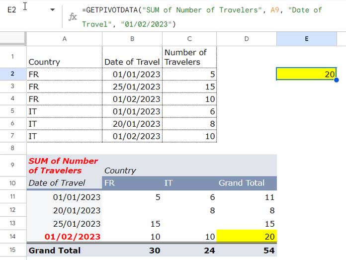
Formula Explanation:
The formula follows the below syntax:
GETPIVOTDATA(value_name, any_pivot_table_cell, [original_column, …], [pivot_item, …])Where:
- GETPIVOTDATA: Retrieves a value from a Pivot Table.
- “SUM of Number of Travelers” (
value_name): This is the name of the data field you want to retrieve, along with the specific aggregation (in this case, the sum) used in the Pivot Table. - A9 (
any_pivot_table_cell): This refers to the top-left cell of the Pivot Table. - “Date of Travel” (
original_column): Name of the source data column used for filtering. - “01/02/2023” (
pivot_item): Date criterion for filtering. Match the format used in the source data.
Key Points:
- Adjust cell references and field names based on your Pivot Table structure.
- Ensure consistent date formats between the formula and source data.
When using a cell reference for the pivot_item criterion (e.g., G2), present it as text using one of these methods:
- TEXT function:
TEXT(G2, "DD/MM/YYYY")(adjust format as needed). - Apostrophe:
'before the date. - Format as Plain Text:
Apply Format > Number > Plain Textto the cell.
Example 2 (Manual Date Grouping and Filter by Rows)
(Refer to Sheet2 in the Sample Sheet above)
Here, let’s utilize the existing Pivot Table with date grouping.
To manually group dates by month in the Pivot Table:
- Right-click on any date in the Pivot Table cell range A11:A14.
- Choose “Create pivot date group” > “Month.”
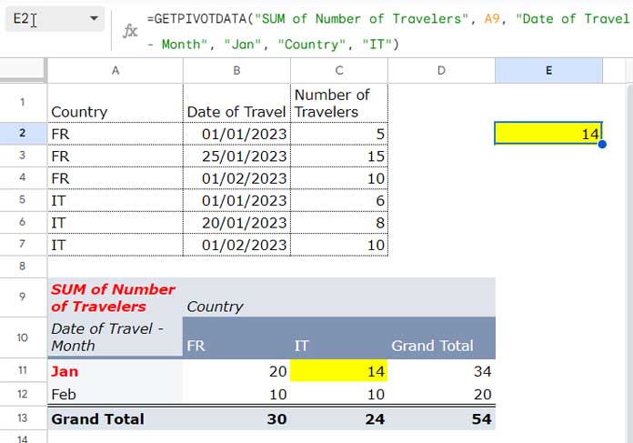
To extract the number of travelers to Italy (IT) in January, use this formula:
=GETPIVOTDATA("SUM of Number of Travelers", A9, "Date of Travel - Month", "Jan", "Country", "IT")The formula yields the total number of travelers to Italy in January.
Explanation:
- GETPIVOTDATA: Retrieves a value from a Pivot Table.
- “Sum of Number of Travelers” (
value_name): Specifies the column header in the Pivot Table, indicating the name of the data field you want to retrieve. - A9 (
any_pivot_table_cell): Refers to any cell within the Pivot Table, typically the top-left cell. - “Date of Travel – Month” (
original_column): Use this name as it reflects the grouped date field in the Pivot Table, even though it differs from the source data column name. - “Jan” (
pivot_item): Date criterion for filtering, matching the grouped month name. - “Country” (
original_column): Name of the source data column used for filtering. - “IT” (
pivot_item): Country for filtering.
Key Points:
- When using GETPIVOTDATA with manually grouped dates in Google Sheets, it’s important to use the grouped field name exactly as it appears in the Pivot Table, even if it differs from the source data column name. In this case, we have used “Date of Travel – Month” instead of “Date of Travel” (
original_column). - Match the
pivot_itemfor the date group (“Jan”) to the displayed month name in the Pivot Table. - Adjust cell references and field names based on your actual Pivot Table structure.
Using GETPIVOTDATA with Grouped Dates in Columns in Google Sheets
This time, we will use different Pivot Table settings. (The first 5 steps are the same as above, but I am repeating them to save your time from scrolling up.)
- Move to cell A9.
- Click on “Insert” > “Pivot Table.”
- In the “Data range” field, enter the correct range A1:C7.
- Select “Existing sheet” and enter A9 in the provided field.
- Click “Create” to insert the Pivot Table and open the sidebar Pivot Table editor panel.
- Drag and drop the field “Country” below
Rows. - Drag and drop the field “Date of Travel” under
Columns. - Under
Values, drag and drop the field “Number of Travelers” and ensure that “Summarize by” is set to SUM.
We will test the GETPIVOTDATA function in this Pivot Table both with and without manual date grouping.
Example 1 (Filter by Columns)
(Refer to Sheet3 in the Sample Sheet above)
Even though the layout is different, we can use the same formula as in “Example 1 (Filter by Rows)” to fetch the total number of travelers on 01/02/2023. This is because the Pivot Table starts in cell A9, and we have not used any other cell reference in the Pivot Table in the formula.
The original_column and pivot_item are the same. But just for example purposes, we will use a different filter criterion.
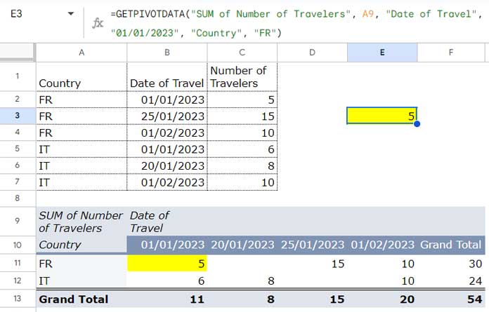
The following formula will return the number of travels to France on “01/01/2023”:
=GETPIVOTDATA("SUM of Number of Travelers", A9, "Date of Travel", "01/01/2023", "Country", "FR")Needless to say, you can use this formula with the Pivot Table used in “Example 1 (Filter by Rows)” to obtain the same result.
Formula Explanation:
- GETPIVOTDATA: Retrieves a value from a Pivot Table.
- “SUM of Number of Travelers” (
value_name): Specifies the column header in the Pivot Table. - A9 (
any_pivot_table_cell): This refers to the top-left cell of the Pivot Table. - “Date of Travel” (
original_column): Name of the source data column used for filtering. - “01/02/2023” (
pivot_item): Date criterion for filtering. - “Country” (
original_column): Name of the source data column used for filtering. - “FR” (
pivot_item): Country for filtering.
Example 2 (Manual Date Grouping and Filter by Columns)
(Refer to Sheet4 in the Sample Sheet above)
Let’s apply manual date grouping and explore how to use the GETPIVOTDATA function with manually grouped dates in columns.
Here as well, the formula used in “Example 2 (Manual Date Grouping and Filter by Rows)” will yield the same result.
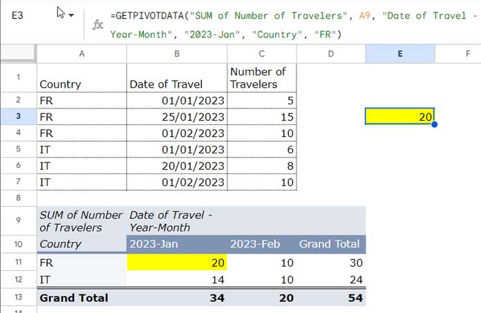
In that case, we applied Month grouping. Here, we will employ a different grouping, namely “Year-Month.”
- Right-click on any date in the above Pivot Table, i.e., “Example 1 (Filter by Columns),” cell range B10:E10.
- Choose “Create pivot date group” > “Year-Month.”
Formula:
=GETPIVOTDATA("SUM of Number of Travelers", A9, "Date of Travel - Year-Month", "2023-Jan", "Country", "FR")This formula will return the number of travels in January 2023 to France.
If you group the Pivot Table in “Example 2 (Manual Date Grouping and Filter by Rows)” by Year-Month instead of Month and apply the same formula above, you will obtain the same result.
Formula Explanation:
- GETPIVOTDATA: Retrieves a value from a Pivot Table.
- “Sum of Number of Travelers” (
value_name): Specifies the column header in the Pivot Table. - A9 (
any_pivot_table_cell): Refers to any cell within the Pivot Table, typically the top-left cell. - “Date of Travel – Year-Month” (
original_column): Use this name as it reflects the grouped date field in the Pivot Table. - “2023-Jan” (
pivot_item): Date criterion for filtering, matching the grouped Year-Month name. - “Country” (
original_column): Name of the source data column used for filtering. - “FR” (
pivot_item): Country for filtering.
Key Takeaways for GETPIVOTDATA with Grouped Dates
GETPIVOTDATA is a highly useful tool for retrieving values from a Pivot Table. It can be employed with the date field grouped in either rows or columns in the same manner. The formula remains unchanged when the layout undergoes modifications.
However, it is crucial to ensure that the Pivot Table is not relocated when adjusting the layout. If you move it to a different range, you need to correctly specify the any_pivot_table_cell argument in the formula. No other changes are required.
Here are the key takeaways for using GETPIVOTDATA with grouped dates in Google Sheets:
- You need to correctly specify the
original_columnandpivot_itemarguments based on the date grouping. - If no manual date grouping is applied, use the
original_column, in our case “Date of Travel,” as the original column and any unique date from this column as thepivot_item, but in the same date format. - If manual date grouping is applied, use the
original_columnas it appears in the Pivot Table, and also use thepivot_itemcriterion accordingly.
Resources:


