When dealing with large numbers in financial data, you may want to format numbers in either thousands, millions, or a combination of both. Custom number formatting is the best way to achieve this in Google Sheets.
However, this approach has its limitations as it applies to predefined cell ranges. But what about the output of a formula that may increase in size both horizontally and vertically over time?
You might consider using CHOOSECOLS or INDEX to extract columns from the formula result and apply text formatting.
While this approach may work to some extent, it’s important to note that it converts numbers to text. Additionally, you might need some expertise to extract columns from a multi-column output, format them, and stack them.
As a result of formatting to text, you may encounter issues when using the processed data in further calculations.
However, this doesn’t mean that there is only one option to format numbers in thousands or millions in Google Sheets without altering the underlying value.
You can use the QUERY function, similar to the TEXT function, to format numbers while retaining the underlying value in number format.
Formatting numbers in millions or thousands in charts is also possible.
Formatting Numbers to Thousands (K) in Google Sheets
We will begin with the Custom number format, which is the preferred method for formatting numbers into thousands or millions in Google Sheets.
In custom number formats, # and 0 serve as number placeholders and a comma is used as the thousand separator. In this, # represents a digit (0-9) that will be displayed if there is a non-zero digit in that place value, while 0 represents a digit that will always be displayed, even if it’s zero.
If you omit any placeholder after the thousand separator, the number will be abbreviated to thousands.
Please refer to the table below to select the appropriate format string for formatting numbers into thousands (K) in Google Sheets.
| Numbers to Format -> | 1500 | 1500.25 | 14500 | 145001 | 2500000 |
| Format Strings ↓ | Result | Result | Result | Result | Result |
| #,##0, | 2 | 2 | 15 | 145 | 2,500 |
| #,##0.0, | 1.5 | 1.5 | 14.5 | 145.0 | 2,500.0 |
| #,##0.0,”K” | 1.5K | 1.5K | 14.5K | 145.0K | 2,500.0K |
| #,##0,”K” | 2K | 2K | 15K | 145K | 2,500K |
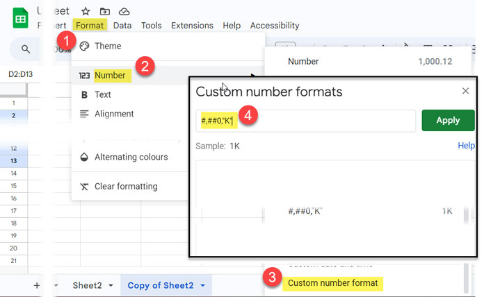
For example, we can apply #,##0,"K" to the range D2:D13 by following these steps in Google Sheets:
- Select the cell range D2:D13.
- Click Format > Number > Custom number format.
- In the Custom number format field, enter the following format string:
#,##0,"K" - Click Apply.
The numbers in the selected cells are now formatted in thousands with the number format #,##0,"K". Here is a screenshot of the result.
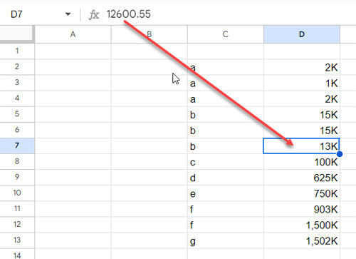
Please note that there have been no changes in the underlying value of the cells.
Using Formulas
We can use QUERY or the TEXT function to format numbers into thousands in Google Sheets.
When using the TEXT function, it returns the numbers in text format, while the QUERY function retains the underlying values as numbers.
Which one should you choose?
So, if you prefer not to use the Custom Number Format due to flexibility issues, you can use either the TEXT or QUERY functions.
The difference lies in the underlying values in the result cells. The TEXT function returns text values, whereas the QUERY function preserves the original numbers.
Therefore, I would recommend using the QUERY function to format numbers into thousands if you prefer a formula over the Custom number format.
Scroll up and select the format string from Table #1 that suits your needs. Below is an example of how to use the number formatting in these functions.
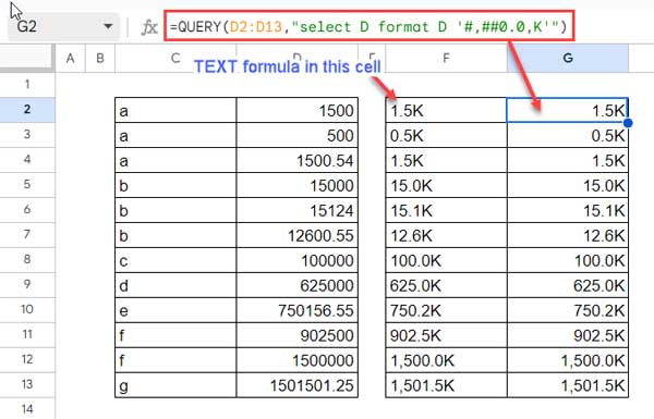
TEXT Formula (for the range B2:B13):
=ArrayFormula(TEXT(D2:D13,"#,##0.0,K"))QUERY Formula (for the range B2:B13):
=QUERY(D2:D13,"select D format D '#,##0.0,K'")Points to Note:
- In both functions, you must remove the double quotes around
Kin the format string. - In the TEXT function, the format string must be placed within double quotes, whereas in QUERY, it should be within single quotes.
Formatting Numbers to Millions (M) in Google Sheets
Please refer to the table below to select the appropriate format string for formatting numbers into millions (M) in Google Sheets.
| Numbers to Format -> | 155699 | 1000000 | 1450055 | 5603200 | 56550212 |
| Format Strings ↓ | Result | Result | Result | Result | Result |
| #,##0,, | 0 | 1 | 1 | 6 | 57 |
| #,##0.0,, | 0.2 | 1.0 | 1.5 | 5.6 | 56.6 |
| #,##0.0,,”M” | 0.2M | 1.0M | 1.5M | 5.6M | 56.6M |
| #,##0,”M” | 0M | 1M | 1M | 6M | 57M |
How does this differ from the number formats used for showing numbers in thousands?
In this format, there are two commas immediately after the last number placeholder: one comma is equivalent to dividing the number by 1,000, whereas two commas are equivalent to dividing the number by 1,000,000.
Another change is replacing the letter ‘K’ with ‘M.’
I’ve already explained how to apply a custom number format to a selected cell range above, with a supporting screenshot. Here’s a quick summary to save you from scrolling up:
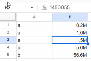
To apply the format #,##0.0,,"M" to the range B1:B5, follow these steps:
- Select the range.
- Click on Format > Number > Custom number format.
- Copy and paste the provided format string into the field.
- Click Apply.”
Using Formulas
We can use the TEXT function or the QUERY function to format numbers into millions in Google Sheets. However, when using these formulas, simply copy-pasting the format string won’t work; you need to make a few changes. Here they are:
In both functions, you must remove the double quotes around M.
The letter M won’t work, as it might be interpreted as a time component. Instead, you should replace it with an alternative letter, Μ, which you can obtain by inserting the following CHAR formula in any blank cell: =CHAR(924)
In the TEXT function, the custom number format must be placed within double quotes, whereas in QUERY, it should be within single quotes.
Here are examples of using the TEXT and QUERY functions to display the numbers in cells B1:B5 in millions.
TEXT Formula (for the range B1:B5):
=ArrayFormula(TEXT(B1:B5,"#,##0.0,,Μ"))QUERY Formula (for the range B1:B5):
=QUERY(B1:B5,"select B format B '#,##0.0,,Μ'")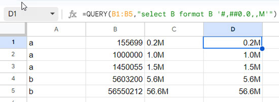
Please note that the TEXT function returns text, whereas the QUERY function returns numbers.
Dynamic Formatting Numbers to Millions and Thousands in Google Sheets
It’s impractical to apply the numbers-to-thousands or numbers-to-millions format mentioned above to a range of cells when there is a significant difference between two numbers. For example, formatting 10,000 to millions may result in 0.0M. To address this, we may need to conditionally format the numbers:
Numbers below 1,000,000 in thousands and those above in millions. This is achievable in Google Sheets using both Custom number format and TEXT/QUERY formulas.
Note: Since we apply conditions, 0 and negative numbers won’t be converted. They will retain their original format and be highlighted in red.
Here is the format string to dynamically convert number formatting to thousands or millions in Google Sheets.
[>=1000000] #,##0.0,,"M";[>0] #,##0.0,"K";[Red]GeneralYou can apply it to the selected range as follows:
To apply to the range A1:A5, follow these steps:
- Select the range A1:A5.
- Click on Format > Number > Custom number format.
- Copy and paste the provided format string into the field.
- Click Apply.”
Here are the corresponding formula options.
TEXT:
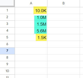
=ArrayFormula(TEXT(A1:A5,"[>=1000000] 0.0,,Μ;[>0] 0.0,K;General"))QUERY:
=QUERY(A1:A5,"Select A format A '[>=1000000] 0.0,,Μ;[>0] 0.0,K;General'")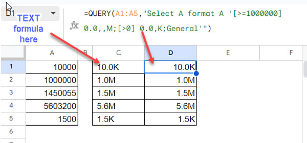
Formatting Numbers to Millions or Thousands in Charts
We can format numbers in thousands or millions for chart axis labels or data point labels. This can help reduce the space required for labeling within the chart.
The easiest way to format numbers in millions or thousands in a Google Sheets chart is as follows:
Double-click on the axis or data point labels. Here, I’ll start by changing the number format of the vertical axis.
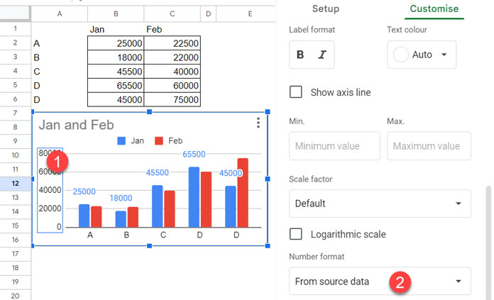
Under “Number format,” click the dropdown and select “Other custom formats.”
Copy and paste one of the format strings from the tables above, then click “Apply.”
Next, double-click on the data point labels.
Select the custom number format as before and paste the copied format string.
Click “Apply.”
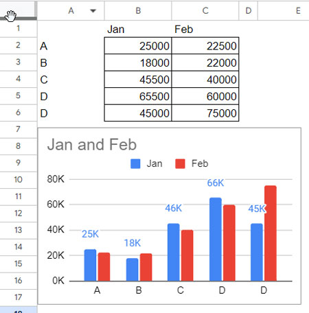
In the above chart, I’ve only enabled data point labels for one series. If you have two series, you will need to repeat the number formatting for both separately.
That’s all. Thank you for reading. Enjoy.


