You can use either custom number formatting or the TEXT function to format numbers as fractions in Google Sheets.
Fractions consist of two numbers separated by a “/” symbol. For example, in 1/2, 1 is the numerator and 2 is the denominator. The numerator indicates how many parts you have, while the denominator shows how many equal parts the whole is divided into.
If you enter a fraction less than one in a cell in Google Sheets, it may be converted to a date, which you might not immediately recognize unless you check the underlying value in the formula bar. If the fraction is greater than one, it will typically be displayed as text.
This is where formatting numbers as fractions in Google Sheets becomes important.
In Excel, there is a specific option in the Format Cells dialog (Ctrl+1) called “Fraction,” but this option is not available in Google Sheets.
Google Sheets users need to use “Custom number format” to display numbers as fractions while retaining the numeric formatting.
Two Ways to Format Numbers as Fractions in Google Sheets
You can format numbers as fractions in two ways:
- Using Custom Number Formatting
- Using the TEXT Function
The first method retains the number format, while the second converts the number to a text string. Note that the formula (second method) will return the result in a helper cell or range.
1. Using Custom Number Formatting
- Select the cell or cell range containing the number(s) you want to format as fractions.
- Click Format > Number > Custom number format.
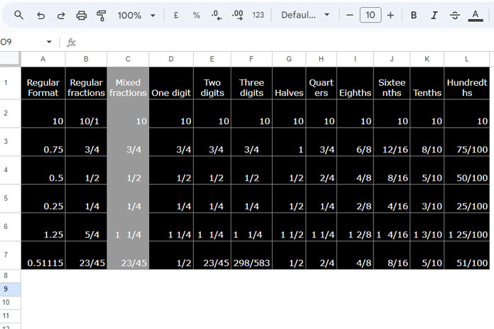
- In the “Custom number format” field, you can use the following formats:
- Regular fractions:
_# ??/??
Displays fractions with up to two digits in both the numerator and denominator. - Mixed fractions:
# ??/??(Recommended)
Shows whole numbers with fractions; suitable for most mixed number representations. - One digit:
# ?/?
Displays fractions with a single digit in the numerator and denominator. - Two digits:
# ??/??
Shows fractions with up to two digits in both the numerator and denominator. - Three digits:
# ???/???
Displays fractions with up to three digits in both the numerator and denominator. - Halves:
# ?/2
Formats numbers as fractions with a denominator of 2 (halves) - Quarters:
# ?/4
Formats numbers as fractions with a denominator of 4 (quarters) - Eighths:
# ?/8
Formats numbers as fractions with a denominator of 8 (eighths) - Sixteenths:
# ??/16
Formats numbers as fractions with a denominator of 16 (sixteenths) - Tenths:
# ?/10
Formats numbers as fractions with a denominator of 10 (tenths) - Hundredths:
# ??/100
Formats numbers as fractions with a denominator of 100 (hundredths)
2. Using the TEXT Function
Here are a few examples of formatting numbers as fractions using the TEXT function in Google Sheets.
Syntax:
TEXT(number, format)In the format argument, you can use one of the formats from the list provided above.
Assume the cell range A1:A6 contains the following data:
| A |
| 10 |
| 0.75 |
| 0.5 |
| 0.25 |
| 1.25 |
| 0.51115 |
In cell B1, enter the following formula and drag it down to B6 to format these numbers as mixed fractions:
=TEXT(A1,"# ??/??")| A | B |
| 10 | 10 |
| 0.75 | 3/4 |
| 0.5 | 1/2 |
| 0.25 | 1/4 |
| 1.25 | 1 1/4 |
| 0.51115 | 23/45 |
Refer to the list above to use the format that best fits your needs.
Real-Life Uses of Formatting Fractions with TEXT
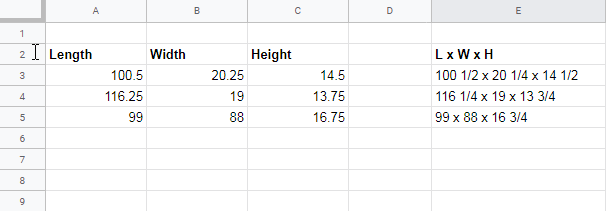
I have a measurement sheet with length, width, and height values in columns A, B, and C, respectively (range is A3:C5). I want to format these measurements as fractions and combine them in column E (E3:E5).
Step 1:
Enter the following formula in cell E3 to format the length, width, and height as fractions:
=TEXT(A3, "# ??/??") & " x " & TEXT(B3, "# ??/??") & " x " & TEXT(C3, "# ??/??")You can either drag this formula down or convert it to an array formula using the following:
Step 2:
To apply this formula to multiple rows, use the ARRAYFORMULA function to expand it down the column:
=ARRAYFORMULA(TRIM(TEXT(A3:A5, "# ??/??") & " x " & TEXT(B3:B5, "# ??/??") & " x " & TEXT(C3:C5, "# ??/??")))This formula formats each measurement as a fraction and combines them with ” x ” as the separator. The TRIM function is used to remove any extra spaces.
Resources
- How to Set Your Country’s Currency Format in Google Sheets
- Currency Formatting in Google Sheets Drop-Downs
- Format Numbers as Currency Using Formulas in Google Sheets
- Formatting Date, Time, and Numbers in Google Sheets Query
- How to Format Query Pivot Header Row in Google Sheets
- How to Concatenate a Number without Losing Its Format in Google Sheets
- Convert Date Format from Dot to Slash or Hyphen in Google Sheets
- How to Format Time to Millisecond Format in Google Sheets
- How to Convert Seconds to HH:MM:SS Format in Google Sheets
- How to Sort Numbers Formatted as Text in Google Sheets (Formula Approach)
- How to Get the Split Result in Text Format in Google Sheets
- Format a Date Without Converting it Into a Text – Google Sheets
- Format Numbers To Millions and Thousands in Google Sheets


This helped me to be able to type fractions into a cell but now I want to add those fractions. The sum function doesn’t seem to work with adding the fractions. Any ideas? Google doesn’t even know lol.
Hello…
I used this method to get the format to display a fraction, thank you.
However, some of the fractions I’m displaying are negative (they are railing lengths and if the resulting fraction is negative it is too long for the given space if the fraction is positive it is too short for the given space).
So if my cell generates a negative number, for example, -0.125, can I get this to display -1/8? Currently, it displays 1/8 without the negative. Thanks.
My workaround is – I used conditional formatting to format each negative value in red, so even though the cell displays -0.125, and then 1/8, conditional formatting picks up on the fact it is a negative value and formats all my cells properly.
Hi, Tom,
A number format pattern is in the following order.
[POSITIVE NUMBER FORMAT];[NEGATIVE NUMBER FORMAT];[ZERO FORMAT];[TEXT FORMAT]So you can try using the following format for negative/positive fractions.
# ?/?;-# ?/?Thanks for sharing the conditional format workaround.
thank you so much…….