To find unmatched records similar to an anti-join, you can use a combination of FILTER, NOT, IFNA, and XMATCH functions in Google Sheets. Google Sheets doesn’t directly support anti-joins as a built-in function.

An anti-join, also called a left anti-join, aims to find records in the left table that have no matching records in the right table. In contrast, a left join retrieves records from the left table and the matching records from the right table.

We will follow the approach below to find unmatched rows in Google Sheets:

• XMATCH: Match the unique IDs in the left table with those in the right table. This function returns the relative position for matches and #N/A for mismatches.
• IFNA: Replace #N/A errors from XMATCH with a more manageable value.
• NOT: Return TRUE for mismatches and FALSE for matches.
• FILTER: Filter the rows where the condition is TRUE.

Anti-Join with One Column: Find Unmatched Records Based on a Single Column

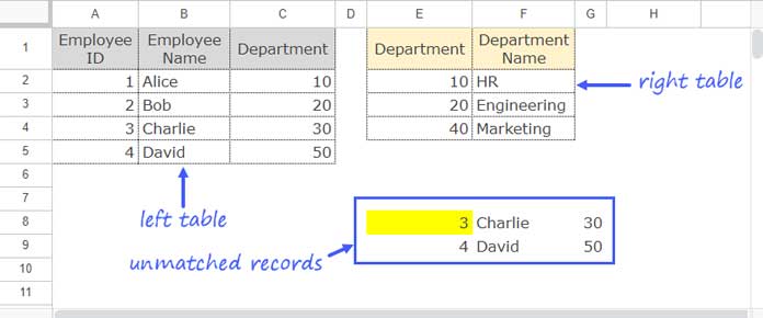
In the following example, the first table contains employee IDs, their names, and their department IDs. The data range is A1:C5.

The second table contains department IDs and department names. The data range is E1:F4.

Match the department IDs in the first table (left table) with those in the second table (right table) and find the unmatched records in the first table.

Formula:

=LET(table1, A2:C5, table1ID, C2:C5, table2ID, E2:E4, FILTER(table1, NOT(IFNA(XMATCH(table1ID, table2ID)))))

When you use this formula, replace A2:C5 with the reference for the left table, C2:C5 with the column reference representing values from the left table that will be matched against the right table, and E2:E5 with the column reference in the right table containing values to match.

This example demonstrates how to perform an anti-join with one column in Google Sheets. It is useful for finding unmatched records by matching values in a unique identifier column in both tables.

Formula Breakdown

FILTER(table1, NOT(IFNA(XMATCH(table1ID, table2ID))))

This follows the FILTER function syntax FILTER(range, condition1, [condition2, …]).

Where:

• range: table1, i.e., the left table range.
• condition: NOT(IFNA(XMATCH(table1ID, table2ID)))

Explanation:

• XMATCH: Matches values in table1ID with table2ID and returns the relative position for matches and #N/A for mismatches.
• IFNA: Replaces #N/A errors with empty values.
• NOT: Converts relative positions (from XMATCH) to FALSE and empty values (returned by IFNA) to TRUE.
• FILTER: Filters rows where the condition NOT(IFNA(XMATCH(table1ID, table2ID))) is TRUE, indicating unmatched records.

This formula extracts rows in table1 that do not have corresponding matches in table2, based on the specified columns (table1ID and table2ID).

We have assigned names to ranges and used those names in the formula, made possible by the LET function.

Anti-Join with Two Columns: Find Unmatched Records Based on Multiple Columns

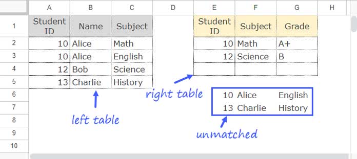
This time, we have student IDs, their names, and subjects in the left table, and student IDs, subjects, and grades in the right table. The table ranges are A1:C5 and E1:G3, respectively.

Here, we aim to match student IDs and subjects from the left table with those in the right table and extract the mismatched records.

Formula:

=LET(table1, A2:C5, table1ID, TRANSPOSE(QUERY(TRANSPOSE({A2:A5, C2:C5}), ,9^9)), table2ID, TRANSPOSE(QUERY(TRANSPOSE({E2:E3, F2:F3}), ,9^9)), FILTER(table1, NOT(IFNA(XMATCH(table1ID, table2ID)))))

When you use this formula to find unmatched records based on multiple columns, make the following changes:

• Replace A2:C5 with the reference for the left table.
• Replace the ranges in the array {A2:A5, C2:C5} with the references to the columns in the left table. Values in these columns will be concatenated for matching in the right table.
• Replace the ranges in the array {E2:E3, F2:F3} with the references to the columns in the right table. Values in these columns will be concatenated for matching.

If you have another identifier column or additional columns to include in the matching process, you can specify them within the respective arrays as needed.

Formula Explanation

This formula aligns with our previous example demonstrating how to perform an anti-join using one column for matching.

The key distinction here lies in defining table1ID and table2ID.

In this scenario, we execute an anti-join based on multiple columns, utilizing XMATCH for matching purposes, even though it doesn’t inherently support multi-column matching.

To accomplish this, we employ the TRANSPOSE-QUERY-TRANSPOSE combination to concatenate columns for comparison.

table1ID is derived from TRANSPOSE(QUERY(TRANSPOSE({A2:A5, C2:C5}), ,9^9)).

The TRANSPOSE function adjusts the data orientation, converting rows into columns. The QUERY function concatenates values from each column into a single combined value, treating all values as headers. Another TRANSPOSE reverts the orientation, resulting in a single-column output.

The same process applies to table2ID, which transforms two columns into a single combined column for comparison.

Resources

We have explored the anti-join (also known as left anti-join) in Google Sheets. Here are some resources related to joining two tables in Google Sheets:

• Merging Two Tables in Google Sheets: The Ultimate Guide
• How to Left Join Two Tables in Google Sheets
• How to Right Join Two Tables in Google Sheets
• How to Inner Join Two Tables in Google Sheets
• How to Full Join Two Tables in Google Sheets
• Master Joins in Google Sheets (Left, Right, Inner, & Full) – Duplicate IDs Solved