Many of us use calendars in Google Sheets to record events. But how do you filter today’s or any particular day’s events from a calendar layout in Google Sheets?

Of course, it’s easy to filter today’s events when the data is in tabular form, such as dates in one column and events in another.

For example, consider dates in column A and events in column B. You can use the following filter formula to filter today’s events:

=FILTER(B1:B, A1:A=TODAY())

However, when you have events entered in a calendar layout, this approach won’t work because dates are spread across multiple rows, arranged week-wise.

Example of Filtering Today’s Events from a Calendar Layout in Google Sheets

To filter today’s events from a calendar, you must ensure one thing:

The dates in the calendar must be proper date values, not just numbers like 1, 2, …, 31. Some users may apply custom number formatting to display dates as day numbers, which is fine. If you have a start date in one cell (e.g., A1) and use A1+1 to get the next date, that is also considered valid date data.

If you don’t have such a calendar, you can copy my template using the button below.

Calendar Template

To use it, enter the month name in cell H1 and the year in cell I1. The calendar will update with dates corresponding to that month and year.

In the following example, I have a calendar in the range C3:I22 with events entered below some of the dates.

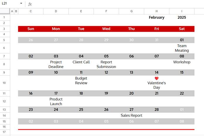
The first row contains the names of the days of the week, followed by one empty row. Then, each week’s dates appear in corresponding rows, separated by one empty row for entering events.

To filter events that fall on today’s date from this calendar, enter the following formula in cell K3:

=LET(
   calendar, C3:I16, 
   calendar_start, C3, 
   height, 1, 
   rows, TOROW(BYCOL(calendar, LAMBDA(c, XMATCH(TODAY(), c))), 3), 
   cols, TOCOL(BYROW(calendar, LAMBDA(r, XMATCH(TODAY(), r))), 3), 
   OFFSET(calendar_start, rows, cols-1, height)
)

How to Use This Formula

• Replace C3:I16 (calendar) with your calendar range.
• Replace C3 (calendar_start) with the first cell of the calendar range.
• Replace 1 (height) with the number of rows between each week’s dates.

The only requirement is that the number of rows between each week must remain consistent. The above formula assumes it is 1 row.

Formula Explanation

Part 1: Find the row position of today’s date in the calendar layout

TOROW(BYCOL(calendar, LAMBDA(c, XMATCH(TODAY(), c))), 3)

• BYCOL scans each column in the calendar for today’s date, returning the row position where it matches and #N/A elsewhere.
• TOROW removes errors and extracts the row position.

Part 2: Find the column position of today’s date in the calendar layout

TOCOL(BYROW(calendar, LAMBDA(r, XMATCH(TODAY(), r))), 3)

• BYROW scans each row for today’s date, returning the column position where it matches and #N/A elsewhere.
• TOCOL removes errors and extracts the column position.

Final Step: Use OFFSET to extract today’s events

OFFSET(calendar_start, rows, cols-1, height)

• We subtract 1 from cols since 0 represents the current column in OFFSET.

What About Filtering Events on Any Specific Date?

Filtering events for a specific date is straightforward once you understand how to filter today’s events.

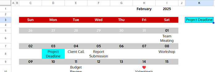
In the formula, replace TODAY() (which appears twice) with the specific date you want.

For example, to filter events on February 3, 2025, replace TODAY() with DATE(2025, 2, 3), using the syntax DATE(year, month, day). The modified formula would be:

=LET(
   calendar, C3:I16, 
   calendar_start, C3, 
   height, 1, 
   rows, TOROW(BYCOL(calendar, LAMBDA(c, XMATCH(DATE(2025, 2, 3), c))), 3), 
   cols, TOCOL(BYROW(calendar, LAMBDA(r, XMATCH(DATE(2025, 2, 3), r))), 3), 
   OFFSET(calendar_start, rows, cols-1, height)
)

Resources

• Convert Google Sheets Calendar into a Table
• Filter a Custom Made Calendar with Events to a New Sheet in Google Sheets
• Hyperlink Calendar Dates to Events in Google Sheets
• Highlighting Today and N Cells Below in Google Sheets Calendar
• Sales Calendar with Top 3 Highlighting in Google Sheets (Template)
• Calendar View in Google Sheets (Custom Template)
• How to Count Events in Particular Time Slots in Google Sheets
• How to Highlight Recurring Event or Payment Dates in Google Sheets
• Highlight Earliest Events Based on Date Column in Google Sheets
• Reservation and Booking Status Calendar Template in Google Sheets
• Dynamic Yearly Calendar Template in Google Sheets: Free Template and How-To Guide
• Fully Flexible Fiscal Year Calendar in Google Sheets
• Create Monthly Calendars in Google Sheets (Single & Multi-Cell Formulas)