When working with Google Sheets, you may encounter blank cells that need to be filled with the nearest non-empty value from below. Unlike the more common top-down fill method, this approach pulls data upward—making it useful for structured datasets, reports, and cleaning up imported data.
In this tutorial, you’ll learn how to fill blank cells with the next non-empty value automatically using built-in Google Sheets functions. Whether you’re dealing with missing labels, structured tables, or gaps in your data, this method will save you time and effort—without manual dragging.
Formula to Fill Blank Cells with the Next Non-Empty Value
Google Sheets provides a formula-based approach to automatically fill empty cells with the next available value below. Here’s how:
=ArrayFormula(XLOOKUP(ROW(range), ROW(range)*(range<>""), range, "", 1, 1))When using this formula, replace range with the actual column reference containing your data.
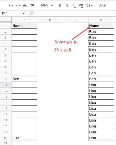
Example: Auto-Fill Blank Cells with the Next Non-Empty Value
Assume you have a list of names in column A with blank cells in between. To fill those blank cells with the next available name, enter this formula in any empty column, ideally in the same row as your dataset:
=ArrayFormula(XLOOKUP(ROW(A1:A), ROW(A1:A)*(A1:A<>""), A1:A, "", 1, 1))This will automatically pull data upward, filling all blank cells with the next non-empty value.
How This Formula Works
This formula uses XLOOKUP, which follows this syntax:
XLOOKUP(search_key, lookup_range, result_range, [missing_value], [match_mode], [search_mode])- search_key:
ROW(A1:A)– Generates row numbers for the given range. - lookup_range:
ROW(A1:A)*(A1:A<>"")– Creates a lookup range that returns the row numbers of non-empty cells. - result_range:
A1:A– The result range containing the values to be returned. - missing_value:
""– Specifies what to return if no match is found (not relevant in this case). - match_mode:
1– Matches the next greater row number when an exact match is not found. This is key to filling blank cells with the next non-empty value. - search_mode:
1– Searches from top to bottom.
Frequently Asked Questions
1. Can I fill blank cells in Google Sheets without dragging?
Yes! This formula automatically fills empty cells without manual dragging or copy-pasting.
2. Does this method work for numbers as well as text?
Absolutely. You can use this technique for both text and numerical values in Google Sheets.
3. What if my data has gaps at the bottom?
If there are blanks at the bottom of your dataset, they will remain empty because there is no lower value to pull from.


