When you drag a formula right and want to increment the cell or range reference down, you can use a versatile formula in Google Sheets. It combines OFFSET and COLUMN functions, and I’ll include the LET function to make it more user-friendly.
Usually, when you drag a formula across (to the right) in Google Sheets, the vertical reference doesn’t increment.
For example, if you enter =A1 in any cell and drag it across to the next column, it will become =B1, not =A2.
Similarly, if you drag =AVERAGE(B2:B3) to the right, it will become =AVERAGE(C2:C3), not =AVERAGE(B3:B4).
If you use absolute references like $B$2:$B$3 or mixed references like $B2:$B3, the reference will remain the same for the rows and columns specified. This is how cell references behave when dragged across columns.
Our OFFSET and COLUMN formula can handle this effectively.
Drag Formula Right, Increment Cell Reference Down: Generic Formula
This is a generic formula and won’t work on its own.
=LET(
   range_start, x, n_rows, y, n_col, z,
   result, OFFSET(range_start, COLUMN(A1)-1, 0, n_rows, n_col),
   result
)
Here are the changes you should make to adapt this formula to your requirements:
range_start: Replacexwith the starting cell of the range. For example, if you want to drag across and get the cell reference down inB2:B, specify$B2.n_rows: Setyto 1 if you want to drag across and increment by one cell.n_col: Setzto 1 if the range contains one column.- For multiple rows: If you want to drag across and increment by two cells down, replace
ywith 2, 3 for three cells, and so on. - For multiple columns: If you want to drag across and include multiple columns, replace
zwith 2 for two columns, 3 for three columns, and so on.
Examples of Dragging a Formula Right While Incrementing Cell References Down
Single Column Range:
Assume you have sales dates in column A and sales values in column B, where A1 and B1 are reserved for field labels.
To get a 2-day rolling average, you might usually use the following formula in cell C3 and drag it down:
=AVERAGE(B2:B3)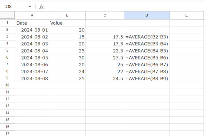
If you want to keep the data orientation the same and get the rolling average across, you can use the following formula:
Step 1: The formula that increments the range down when you drag to the right:
=LET(
   range_start, $B2, n_rows, 2, n_col, 1,
   result, OFFSET(range_start, COLUMN(A1)-1, 0, n_rows, n_col),
   result
)
It increments by two rows and includes 1 column.
Step 2: To get the average, you should wrap result in the above formula with AVERAGE:
=LET(
   range_start, $B2, n_rows, 2, n_col, 1,
   result, OFFSET(range_start, COLUMN(A1)-1, 0, n_rows, n_col),
   AVERAGE(result)
)
Multiple Column Range:
This time we have marks of students in Maths, Physics, and English in columns B to D.
I want the total of each student’s marks to increment by one row down when I drag the formula right, but include three columns.
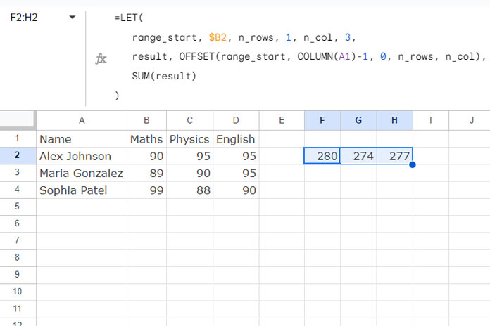
The regular drag-down formula is =SUM(B2:D2) which will become =SUM(B3:D3), =SUM(B4:D4), and so on when we drag down.
How do we get the same result when we drag the formula across?
To achieve this, you can use the following formula that combines the OFFSET and COLUMN functions to handle the row increment and column range:
=LET(
   range_start, $B2, n_rows, 1, n_col, 3,
   result, OFFSET(range_start, COLUMN(A1)-1, 0, n_rows, n_col),
   SUM(result)
)
Formula Explanation
The formula uses the OFFSET function with the following syntax:
OFFSET(cell_reference, offset_rows, offset_columns, [height], [width])We have utilized the LET function to define names for improved readability. In the formula:
range_startrepresents thecell_referenceargument.n_rowsrepresents theheightargument.n_colrepresents thewidthargument.
The offset_rows argument is dynamically specified by COLUMN(A1)-1, which returns a sequence of 0, 1, 2, 3, and so on as you drag across.
This allows the formula to offset by that many rows, which is key for dragging the formula across and incrementing the cell reference down. The n_rows and n_col parameters determine the number of rows and columns in the output.
The offset_columns is set to 0.
Resources
- Shift Column in a Filter Formula When Dragging Down – Google Sheets
- Sum Multiple Columns Dynamically Across Rows in Google Sheets
- Countif Across Columns Row by Row – Array Formula in Google Sheets
- How to Copy Every Nth Cell in a Column in Google Sheets
- Copy-Paste Merged Cells Without Blank Rows/Spaces in Google Sheets


