How to change column letters when a formula is copied down?

I think the title makes sense. I am not going to talk about relative and absolute cell references that using the dollar sign here.

We have already discussed that.

Here I am trying to explain how to change the column letter when a formula is copied down/vertically.

In other words, when dragging down the fill handle of a formula cell, the row position/number should be absolute, but the column position/letter should be relative.

What does it mean?

The formula =A1 should be changed to =B1, =C1, =D1, and so on, when copied to down not right.

Usually, what happens is the formula changes to =A2, =A3, =A4, and so on.

That means I want to change column letters when the formula is copied down in a single column.

Problem to Solve in Detail

See the below example.

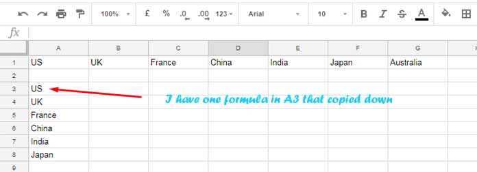
I have a few country names in row # 1 that are in the range A1:G1.

I have a formula (you will get that later) in cell A3 that pointing to cell A1. I’ve copied it to A4, A5, A6, and so on.

Then what happens? It copies the country names in row # 1 down!

Usually, the formula keeps the column heading (column letter) but changes the row number.

For example;

The formula in cell A3 is =A1. Copy this formula to A4. It would be =A2.

But what I want is instead of =A2, I want to get =B1. That’s what I’ve done in the above example.

In other words, I want to change the column letter in the vertical copying of the formula. I want to keep the row number the same but change the column letter.

How to Change Column Letter When Formula Copied Down

Here is that tricky Google Sheets formula that I’ve used in cell A3.

=offset($A$1:1,0,row(A1)-1,1,1)

It’s an Offset formula that dynamically refers to cell A1.

When you copy the above Offset formula down, it refers to B1, C1, D1, and so on, not A2, A3, A4…

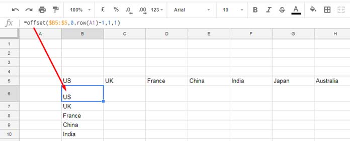
In the above formula, the cell reference is A1. If it’s B5, you should change it as below.

=offset($B5:$5,0,row(A1)-1,1,1)

This formula will return the value from C5, D5, E5, and so on when copied down.

You have got the formula to change column letters only in Google Sheets.

You may be want to know how this Offset based formula works.

If so, you should learn the usage of the functions Offset and Row in Google Sheets.

Feel free to check my useful Google Sheets Functions Guide.

Final Thoughts

I am a great fan of Array Formulas.

But in the above examples, I have not used ArrayFormula instead of a drag-down formula because there is no point in doing so as we have a simple alternative.

Yep, I am talking about TRANSPOSE!

In the last example, the values (texts) that we want to copy down are in the range B5:H5. In an array, you can use this as below.

=transpose(B5:H5)

That’s all.