We can highlight days remaining in two types of Gantt charts in Google Sheets. So we must first know all the available options.

There is no native Gantt Chart item within the menu Insert > Chart in Google Sheets.

So, as far as I know, we can depend on a highlighting rule, Stacked Bar chart, or the SPARKLINE function.

Out of these three, we can’t use the Sparkline function to make the remaining days stand out in the bar because that requires more than two colors.

Usually, we require two colors.

1. Project start to task start – White color.
2. Task start to task end – Any other color.

But to get days remaining in a Gantt chart, we require three colors.

1. Project start to task start – White color (chart background color).
2. Task start to elapsed days (days passed) – Light Orange (any color other than the above).
3. Remaining days – Dark Read (any color other than the above two)

This rules out the possibility of creating a Gantt Chart Using the Sparkline in Google Sheets as it only supports two.

Days Remaining in Gantt Chart – What’s It?

To find the days remaining, we require three parameters. They are the task start date, end date, and today’s date.

In this, the end date is the task deadline.

We should find the number of days from today to the task end date. That is the days remaining to the deadline.

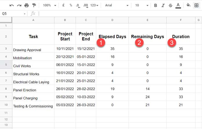
For example, the scheduled duration of the activity “Panel erection” is from 26-01-2022 to 28-02-2022.

If today’s date is 14-02-2022, the remaining days to complete the “Panel erection” is 14, the days elapsed/passed is 19, and the total duration is 33 days.

Data Preparation – Elapsed Days, Remaining Days, and Duration

We require a couple of formulas to achieve our goal. I have explained them below.

From your project schedule, take the input for columns A, B, and C.

We can use MAX, MIN, and TODAY functions based formulas to get the values in the remaining columns.

Here are them.

D3 – Returns the Number of Days Elapsed.

=max(0,days(min(today(),C3),B3))

E3 – Returns the Remaining Days (to reach the deadline).

=max(0,C3-max(today(),B3))

F3 – Duration.

=days(C3:C,B3:B)

You should copy and paste all these formulas up to row # 10.

The above are the essential data formatting to highlight days remaining in a Gantt Chart in Google Sheets.

Note:-

I’ll share my sample Sheet with you at the end of this tutorial. In that, you may see formulas in B3:C10 (under project start and end dates).

That’s to make the sample data evergreen.

You can ignore them completely.

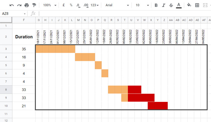
Stacked Bar to Get Days Remaining in Gantt Chart in Google Sheets

Here I’ll share with you the necessary settings only.

You can check my sample sheet at the end of this tutorial to sort out any issues you may face on the course.

Let’s see how to use the Stacked Bar graph to get or display the days remaining in a Gantt chart in Google Sheets.

Must Read: Create GANTT Chart in Google Sheets Using Stacked Bar Chart.

Required Stacked Bar Graph Settings

1. In cell A1 (or in any blank cell), insert =datevalue(min(B3:B10)), which will return the date value of the project start date. We will use it later on.
2. Select A2:E10 and Insert > Chart.
3. Follow the below settings under the Chart editor > Setup tab.
   1. Chart type – Stacked bar chart.
   2. Y-axis – “Task.”
   3. Series – “Project Start,” “Elapsed Days,” and “Remaining Days.”
4. Follow the below settings under the Chart editor > Customize tab.
   1. Under Series, set the “Project Start,” “Elapsed Days,” and “Remaining Days” fill colors to White, Light Orange, and Dark Red, respectively.
   2. Within the same Series, select “Data labels.” Click Number format > Other custom formats and enter "deadline"#0 "days" in the given field and click “Apply.” It’s an optional setting.
   3. Under the Horizontal axis, enter the cell A1 date value, 44510 (or what you get) as per my sample above, in the “Min” field.
   4. Select “Allow boundaries to hide data.”
   5. Click Number format and select “Date and Time.” 

The above is one of the options to get days remaining in the Gantt Chart in Google Sheets.

Highlight Days Remaining in Gantt Chart – Conditional Formatting

If you are comfortable with conditional formatting, you can follow the below method (option) to highlight days remaining in a Gantt chart in Google Sheets.

Here the above “Data Preparation” is not enough. We require a timescale at the top of the bar area, i.e., in G2:AF2.

In G2, insert =min(B3:B10).

In H2, insert =G2+7 and copy-paste to G2:AF2.

You will get a timescale as below.

Note:- Since the timescale contains weeks (7 days), tasks with smaller duration might not appear sometimes.

We are just required to insert two custom rules within Conditional Formatting. Here are them.

Rule 1 (to highlight the days remaining in the Gantt chart bar):

=isbetween(G$2,max(today(),$B3),$C3)

Rule 2 (to get the bar):

=isbetween(G$2,$B3,$C3)

How Do I Apply Them?

Must Read: Create Gantt Chart Using Formulas in Google Sheets.

1. Select G3:AF10.
2. Go to Format > Conditional formatting.
3. Under Format rules, select the custom formula is.
   1. Insert Rule 1 formula, set the fill color to Dark Red, and click Done.
   2. Insert Rule 2 formula, set the fill color to Light Orange, and click Done.

Please make sure that the “Dark Red” rule is above the “Light Orange” rule.

You can drag the rules and place them accordingly.

That’s all. Thanks for the stay. Enjoy!

Sample Charts 15222