Tracking payments in Google Sheets often requires knowing how many days have passed since the last payment. Manually calculating this for each row can be tedious, especially if you’re dealing with months of data. In this guide, I’ll show you how to use an Array Formula in Google Sheets to automatically calculate the days since the previous payment — no dragging formulas down required.
This approach is especially useful for financial trackers, invoices, or subscription records where you need to quickly see gaps between payments.
I’ll cover two approaches:
- A Lambda formula — simple and straightforward, but it may lag with very large datasets.
- A classic array formula — slightly more complex but faster and more reliable for bigger sheets.
Don’t worry, I’ll walk you through both along with explanations.
Sample Scenario
Imagine you maintain a payment log with columns for Date, Amount Due, and Amount Paid. You want Google Sheets to automatically calculate the number of days since the last payment whenever a new entry appears.
Here’s an example table:
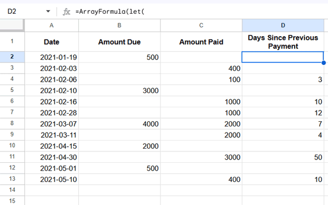
With the right Array Formula, the “Days Since Last Payment” column is filled automatically without any manual work.
Calculate Days Since Last Payment Using MAP + LAMBDA
If your data is in range A1:C, enter this formula in cell D2:
=MAP(
  SEQUENCE(ROWS(A2:A)), A2:A, C2:C,
  LAMBDA(seq, dt, pmt,
    IF(pmt="","",
      IFERROR(
        dt - MAX(FILTER(A2:A, (ROW(A2:A) < seq + ROW(A2)-1) * (C2:C <> ""))),
        ""
      )
    )
  )
)
This formula skips the first payment date. From the second payment onward, it fetches the immediately earlier payment date and subtracts it from the current one. That’s how it calculates the days since the last payment in Google Sheets.
Formula Breakdown
We pass three arrays into MAP:
SEQUENCE(ROWS(A2:A))→ generates sequence numbers from 1 up to the number of rows in the range A2:A.A2:A→ the date range.C2:C→ the payment range.
The LAMBDA assigns these names: seq (sequence number), dt (date), and pmt (payment).
IF(pmt="", "", … )→ skips empty payment rows.MAX(FILTER(A2:A, (ROW(A2:A) < seq + ROW(A2)-1) * (C2:C <> "")))→ finds the most recent payment date before the current row.- Subtracting this from
dtgives the days since the last payment.
Calculate Days Since Last Payment Using a Classic Array Formula
For large datasets, this formula is more efficient. Place it in D2:
=ArrayFormula(let(
   pRows, query(filter(row(A2:A), C2:C>0), "Select * offset 1", 0),
   dt, FILTER(A2:A, C2:C>0),
   array_1, VSTACK(dt, NA()),
   array_2, VSTACK(NA(), dt),
   nd, TOCOL(array_1-array_2, 3),
   IFNA(VLOOKUP(ROW(A2:A), hstack(pRows, nd), 2, 0))
))
This approach calculates all differences at once and then maps them back to the correct rows. It’s slightly harder to read, but it’s faster for long sheets.
Formula Breakdown
pRows→ returns row numbers of payment entries, skipping the first.dt→ filters payment dates.array_1andarray_2→ align shifted payment dates using VSTACK.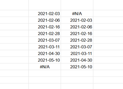
nd→ calculates the differences between consecutive payment dates.- VLOOKUP → assigns those differences back to the correct rows.


