Combine Two Tables with Unequal Rows Horizontally in Google Sheets

When you combine two tables horizontally in Google Sheets, both tables don’t always contain the same number of rows. If you use curly brackets ({}) to combine arrays of unequal heights, Google Sheets returns the following error:

Function ARRAY_ROW parameter n has mismatched row size. Expected: n. Actual: n.

The easiest way to avoid this error is to use HSTACK, which automatically pads the shorter array with #N/A values instead of failing.

In this tutorial, you’ll learn why the error occurs, when it happens, and how to combine tables correctly.

Table of Contents

The Correct Way to Combine Tables with Unequal Rows Horizontally

If you’re combining tables that may contain different numbers of rows, use HSTACK instead of curly brackets.

Note: HSTACK isn’t limited to unequal-sized arrays. It also works perfectly when the arrays have the same number of rows, so you can use it as a drop-in replacement for curly brackets in most horizontal array combinations. The advantage is that your formula continues to work even if one table grows or shrinks later.

Example

Suppose you have two columns of different lengths.

=HSTACK(A1:A10, B1:B5)

Since the second column contains fewer rows, HSTACK automatically pads the remaining rows with #N/A values instead of returning an error.

Remove the #N/A Values

Wrap HSTACK with IFNA if you want blank cells instead of #N/A.

=IFNA(HSTACK(table_1, table_2))

Why Curly Brackets Fail

Curly brackets combine arrays using the undocumented ARRAY_ROW function, which requires every horizontally combined array to contain the same number of rows.

That’s why

={A1:A10, B1:B5}

returns

Function ARRAY_ROW parameter 2 has mismatched row size. Expected: 10. Actual: 5.

Since B1:B5 contains only five rows, Google Sheets cannot align it with the ten-row first array.

Common Situations That Cause the Mismatched Row Size Error

You may not intentionally combine unequal tables, but the error can appear unexpectedly in many real-world situations.

Physical Ranges

Suppose you combine matching columns from two sheets.

={Sheet1!A1:A, Sheet2!A1:A}

If Sheet1 and Sheet2 don’t have the same number of populated rows, the formula returns a #REF! error.

This surprises many users because both references are open-ended. However, Google Sheets compares the actual populated rows, not the range notation.

Use:

=IFNA(HSTACK(Sheet1!A1:A, Sheet2!A1:A))

It works even when the number of rows changes over time.

Named Ranges

Named ranges often change over time.

For example:

={Area, Qty}

If one named range has been expanded but the other hasn’t, their row counts no longer match, causing the error.

Again, HSTACK handles this automatically.

=IFNA(HSTACK(Area, Qty))

Structured Table References

Structured table references can also produce unequal arrays.

For example:

={East[#ALL], North[[#ALL],[Qty]]}

If the two tables contain different numbers of records, the formula fails with the mismatched row size error.

Replace the curly brackets with HSTACK to combine the arrays safely, even when the table sizes change.

New to structured table references? See Structured Table References in Formulas in Google Sheets for a complete introduction before using them in array formulas.

Formula Results

Formula-generated tables frequently return different numbers of rows.

Suppose the following QUERY formulas summarize two datasets.

=QUERY(A1:B,"select A,sum(B) where A is not null group by A",1)

=QUERY(D1:E,"select D,sum(E) where D is not null group by D",1)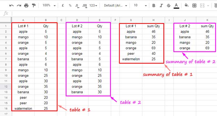

Sample data with two QUERY formulas returning tables of different row counts in Google Sheets

If you combine them like this,

={QUERY(...), QUERY(...)}

the formula fails whenever the two queries return different numbers of rows.

This is one of the most common causes of the error because summary tables rarely return the same number of rows.

Instead, use:

=IFNA(
  HSTACK(
    QUERY(...),
    QUERY(...)
  )
)

This combines both results safely regardless of their sizes.

Summary

When combining tables horizontally:

Use HSTACK whenever the tables might contain different numbers of rows.
Wrap HSTACK with IFNA if you want to hide the automatically inserted #N/A values.
Use curly brackets only when you’re certain every array has exactly the same number of rows.

Following this approach helps you avoid the Function ARRAY_ROW parameter has mismatched row size error while making your formulas more reliable and easier to maintain.

Frequently Asked Questions

Why do curly brackets return the mismatched row size error?

Curly brackets require every horizontally combined array to have the same number of rows. If one array is shorter, Google Sheets returns the ARRAY_ROW parameter has mismatched row size error.

Should I use HSTACK or curly brackets?

Use HSTACK whenever the number of rows may change or is unknown. Curly brackets are suitable only when the arrays are guaranteed to have the same number of rows and you prefer a more concise formula.

How do I combine tables with unequal columns in Google Sheets?

This tutorial covers tables with unequal rows when combining them horizontally. If your tables have different numbers of columns and you want to combine them vertically in a QUERY formula, see Combine Tables with Unequal Columns in Google Sheets QUERY.

Conclusion

Curly brackets are still useful when every array is guaranteed to have the same height. But if the row count can change—as with QUERY, named ranges, structured table references, or data imported from other sheets—HSTACK is the safer choice. It handles unequal arrays automatically, and wrapping it with IFNA produces a clean result without hiding genuine formula errors.