The CLEAN function in Google Sheets helps remove non-printable characters from text. You can use it as a standalone function or combine it with lookup functions and logical tests.

Non-printable Characters in Google Sheets

You might encounter non-printable characters when you copy-paste content from external sources like websites, emails, or document editors. These characters often aren’t visible, as they’re used for formatting purposes.

Examples of non-printable characters you can remove using the CLEAN function in Google Sheets include the horizontal tab, line feed, and carriage return. You can represent them using CHAR(9), CHAR(10), and CHAR(13), respectively.

These invisible characters can affect formulas, sorting, filtering, or visual layout in Google Sheets, even though you can’t see them.

For example, try the following formula:

=JOIN(CHAR(9), "APPLE", "ORANGE")

Replace 9 with 10 or 13 to see different formatting effects.

The CLEAN function in Google Sheets removes only non-printable ASCII (American Standard Code for Information Interchange) characters. It does not remove non-printable Unicode characters that aren’t part of ASCII.

Syntax of the CLEAN Function

CLEAN(text)

• text – The string from which you want to remove non-printable characters.

Note: The input can be hardcoded or a reference to a cell. To clean multiple cells in a range, wrap the function in ARRAYFORMULA.

Example of Using the CLEAN Function

Enter one of the following formulas in a cell, say G1, to generate text containing a non-printable character:

="INFO"&CHAR(10)&"INSPIRED"
=JOIN(CHAR(10), "INFO", "INSPIRED")

This creates an in-cell line break: “INFO” appears on the first line and “INSPIRED” on the second.

To remove the line break using the CLEAN function in Google Sheets, use:

=CLEAN(G1)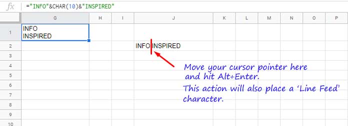

To clean an entire column of text that might include line feed or other non-printable characters, use this formula:

=ARRAYFORMULA(CLEAN(A2:A))

CLEAN vs TRIM in Google Sheets

Many users confuse the CLEAN and TRIM functions. Here’s the difference:

• TRIM removes extra spaces, except for single spaces between words.
• The CLEAN function in Google Sheets removes non-printable characters like line breaks and tabs.

To thoroughly clean up a dataset, you can combine both:

=ARRAYFORMULA(TRIM(CLEAN(A2:A)))

This removes both invisible characters and unwanted spaces.

CLEAN is Useful When Importing Data

If you’re copying data from websites, emails, or PDFs, you might unknowingly bring in hidden formatting. These can break formulas or cause unexpected results.

Use the CLEAN function in Google Sheets to sanitize imported text before using it in formulas or lookups.

CLEAN Doesn’t Remove Non-ASCII Unicode Characters

The CLEAN function only removes the first 32 non-printable ASCII characters. It won’t remove special Unicode characters like non-breaking spaces (CHAR(160)).

You can remove those using REGEXREPLACE:

=REGEXREPLACE(text, CHAR(160), "")

This is helpful when data comes from HTML pages or PDFs.

The Importance of Using CLEAN Function in LOOKUPs and Logical Tests

Non-printable characters can cause lookup formulas to fail. For instance, suppose G1 contains "INFO"&CHAR(10)&"INSPIRED" and you’re trying to match it using:

=XLOOKUP("INFO INSPIRED", G1, H1)

This might not return a match because of the hidden line feed in G1.

Instead, use:

=XLOOKUP("INFO INSPIRED", CLEAN(G1), H1)

This ensures non-printable characters don’t interfere with your lookup results.

Using CLEAN in Array-Based LOOKUPs

If you’re performing lookups across a column with inconsistent formatting, apply CLEAN using ARRAYFORMULA:

=XLOOKUP("INFO INSPIRED", ARRAYFORMULA(CLEAN(G2:G)), H2:H)

This ensures all values are cleaned before lookup, avoiding hidden character mismatches.

Resources

• Pad Values in Google Sheets for Clean Notepad Pasting
• How to Use the TRIM Function in Google Sheets