A calendar week formula in Google Sheets combines the week start and end dates for calendar weeks across a range.
A calendar week refers to a period of seven consecutive days, typically starting on Monday and ending on Sunday.
There is no specific function to directly combine week start and end dates based on calendar weeks. The WEEKNUM function is the only function that identifies calendar weeks, but it returns week numbers rather than week ranges.
What I want is the week start date to end date, such as 04-Feb-2019 to 10-Feb-2019 (Monday-Sunday), rather than just the week number 6 (though we can specify a Sunday-Saturday week as well).
My calendar week formula returns the start and end dates of each week from a list of dates. Additionally, the formula is compatible with date ranges that span different years.
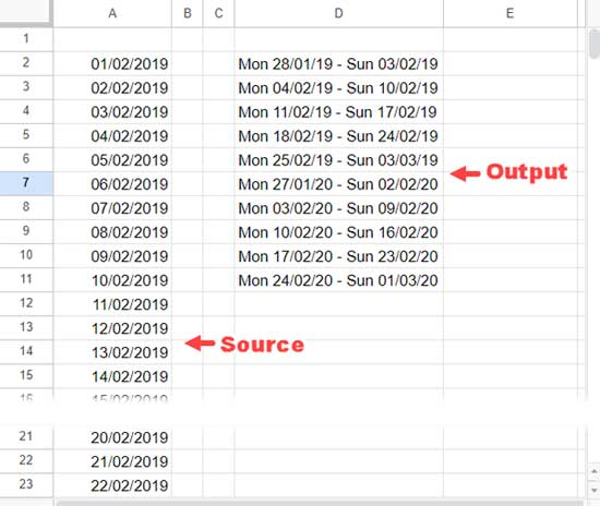
First, review the output produced by my calendar week formula, and then I will explain its applications.

Note: If you want the week range from the lowest date in the range to 6 days ahead, you will need a different formula. Here is the relevant tutorial: Convert Dates to Week Ranges in Google Sheets (Array Formula).
Extract Week Start & End Dates with a Formula
For this purpose, I have entered some sample dates in column A.
- The rows A2:A29 contain dates from 01/02/2019 to 28/02/2019.
- The rows A30:A58 contain dates from 01/02/2020 to 29/02/2020.
I want to demonstrate the multi-year compatibility of my formula, which is why I have included dates spanning two years.
Additionally, the formula is unaffected by the order of the dates, whether they are sorted in ascending, descending, or random order.
Step 1: Find Unique Week Start Dates
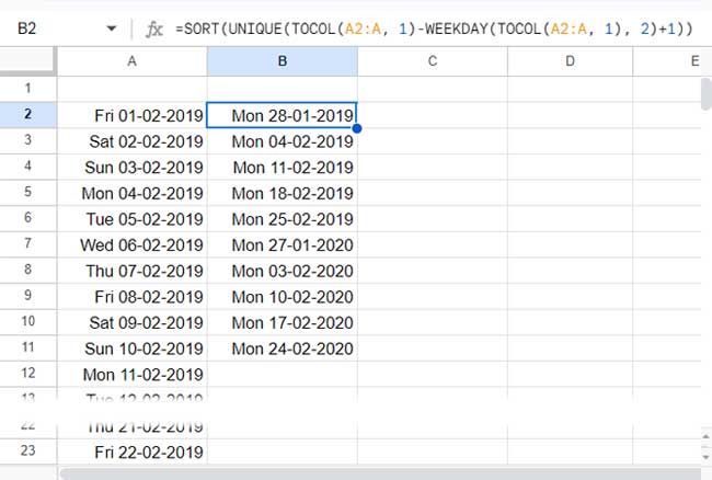
To get the unique calendar week start dates from the range A2:A, enter the following formula in cell B2:
=SORT(UNIQUE(TOCOL(A2:A, 1)-WEEKDAY(TOCOL(A2:A, 1), 2)+1))This formula will place the unique week start dates in B2:B for the dates in all the rows in A2:A.

Explanation:
TOCOL(A2:A, 1): The TOCOL function removes empty cells from the date range.WEEKDAY(TOCOL(A2:A, 1), 2): Removes empty cells from the date range and returns the weekday number of the remaining values.
When you subtract the weekday number from the date and add 1, you get the week start dates for all the dates in A2:A.
- The UNIQUE function returns the unique dates from this result.
- The SORT function sorts the result and also acts as an array function replacement in the formula, as WEEKDAY requires this support.
Please note that I’ve used type #2 within the WEEKDAY function to start the week on Monday. You can specify 1 if you want the week to start on Sunday.
Step 2: Find Unique Week End Dates
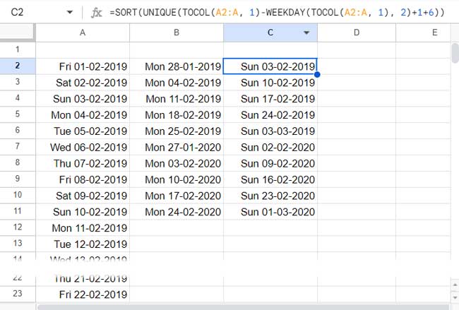
If you add 6 days to the calendar week start date, you will get the calendar week end date. Enter the following formula in cell C2:
=SORT(UNIQUE(TOCOL(A2:A, 1)-WEEKDAY(TOCOL(A2:A, 1), 2)+1+6))
Step 3: Combine Week Start & End Dates
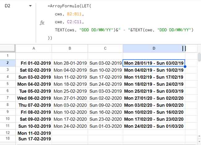
In cell D2, enter the following formula to combine the calendar week start and end dates:
=ArrayFormula(LET(
   cws, B2:B11,
   cwe, C2:C11,
   TEXT(cws, "DDD DD/MM/YY")&" - "&TEXT(cwe, "DDD DD/MM/YY")
))
Explanation:
The LET function assigns the name ‘cws’ to the date range in B2:B11 and ‘cwe’ to the date range in C2:C11. Then, use those names in the formula expression: TEXT(cws, "DD/MM/YY")&" - "&TEXT(cwe, "DD/MM/YY").
Actually, this formula expression could simply be cws&" - "&cwe, combining the calendar week start and end dates. However, doing so would convert the dates to date values. Therefore, we use the TEXT function to get the format DDD DD/MM/YY (you can specify your preferred format, such as DDD MM/DD/YY, as well).
The ARRAYFORMULA is necessary because we are using the TEXT function, which is not an array function, in an array context.
Step 4: Clean Up (Optional)
This step removes helper columns and also improves formula performance. However, it is optional.
In the above formula, replace B2:B11 with the formula in B2 and C2:C11 with the formula in C2.
=ArrayFormula(LET(
   cws, SORT(UNIQUE(TOCOL(A2:A, 1)-WEEKDAY(TOCOL(A2:A, 1), 2)+1)),
   cwe, SORT(UNIQUE(TOCOL(A2:A, 1)-WEEKDAY(TOCOL(A2:A, 1), 2)+1+6)),
   TEXT(cws, "DDD DD/MM/YY")&" - "&TEXT(cwe, "DDD DD/MM/YY")
))
Then remove the B2 and C2 formulas from the respective cells.
This is the calendar week formula to combine week start and end dates in Google Sheets.
We can use the full benefit of LET here to shorten this formula. As you can see, TOCOL(A2:A, 1)-WEEKDAY(TOCOL(A2:A, 1), 2) repeats twice in the formula.
You can name it something like ‘cal’ and use that name as follows:
=ArrayFormula(LET(
   cal, TOCOL(A2:A, 1)-WEEKDAY(TOCOL(A2:A, 1), 2),
   cws, SORT(UNIQUE(cal+1)),
   cwe, SORT(UNIQUE(cal+1+6)),
   TEXT(cws, "DDD DD/MM/YY")&" - "&TEXT(cwe, "DDD DD/MM/YY")
))
Resources
- Finding Week Start and End Dates in Google Sheets: Formulas
- Summarize Data by Week Start and End Dates in Google Sheets
- How to Create a Weekly Summary Report in Google Sheets
- Query to Create Daily/Weekly/Monthly/Quarterly/Yearly Report Summary
- How to Count Orders per Week in Google Sheets: Formula Examples
- Query to Calculate Hours Worked in Week Wise in Google Sheets
- How to Group by Week in Pivot Table in Google Sheets


Hello, In your first screenshot, the formula has calculated the dates perfectly.
What was the formula you have used in D1, E1, etc.?
Hi Sushil,
I have just one calendar week array formula in cell C1 that returns values in C1:L1.
That’s the third formula from bottom to top (just above subtitle Option # 2).
Can I include a “most recent” date where it would post the most recent week of an item that matches a particular value from a selected range (data validation)?
Hi, Ashley,
Please share a sample.
How can I tweak this so that it shows all weeks (even if there were 0 orders for that week)?
Thank you!
Hi, Jordon,
In my calendar week formula, replace the range A2:A58 (it appears four times, so replace all the four) with the below SEQUENCE formula.
sequence(days(max(A2:A58),min(A2:A58))+1,1,min(A2:A58))What does this Sequence do then?
It populates dates from min date in the range A2:A58 to max date in the range A2:A58. So the formula will return all the weeks irrespective of orders.