


The Group By clause in Query sorts the output automatically. It’s ideal in most of the cases. But to avoid auto-sorting of data when using the Query Group By clause, there is no built-in clause in Query. That prompts me to think about a workaround!
I am going to address the below two points in this Query related tutorial.
- How to use the Group By clause in Google Sheets Query.
- How to avoid auto sorting in Query Group By clause.
Screenshot # 1:
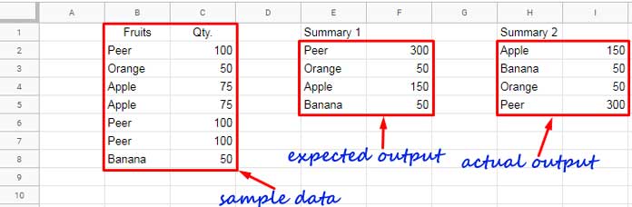
When you use the Group By clause in Query to make the summary of data in B2
I am not telling you that this’s an issue to solve. But by any reason, if you want to return the output that without sorting the items (fruits) then you can use my workaround.
With my workaround, you can avoid auto sorting when using Query Group By clause in Google Sheets. The Query output in the range E2
How to do that? Before proceeding to the workaround first see how to use the Group By clause in Query function in Google Sheets.
How to Use the Query Group By Clause in Google Sheets
To learn how to avoid auto sorting in Query Group By clause, you must know the proper use of this clause and about its auto-sorting.
Must Check: Google Sheets Functions Guide.
The Group By clause in Query is used to aggregate values across rows. A single row is created for each distinct combination of values (groups) in the Group By clause.
As mentioned above the grouped data will be automatically sorted by the grouping columns.
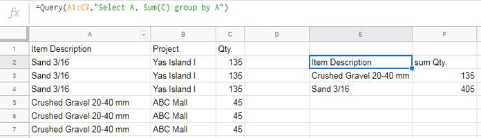
Example 1: Single Column Grouping
=Query(A1:C7,"Select A, Sum(C) group by A")Screenshot # 2:
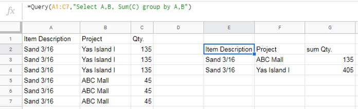
Example 2: Two Column Grouping
=Query(A1:C7,"Select A,B, Sum(C) group by A,B")Screenshot # 3:
In the above examples, I have used the Sum aggregation function in Query. You can use other aggregation functions such as Max, Min, Avg, Count with the Group By clause.
Must Check: How to Sum, Avg, Count, Max, and Min in Google Sheets Query.
When you use the Query Group By clause as above, use only the columns in the Select clause in it.
How to Avoid Auto Sorting When Using Query Group By Clause
I think this time I must use some real-life data. Let’s import a table from this source. The table contains the details of the FIFA World Cup finals.
To import the required data, we can use the IMPORTHTML function. Open a new Google Sheets file. In that enter the below formula in cell A1.
=IMPORTHTML("https://en.wikipedia.org/wiki/List_of_FIFA_World_Cup_finals","table",3)At present, the above formula returns the below table. In any case, if you are unable to import the data, then just type first few rows manually. That will be sufficient for our test.
Screenshot # 4:
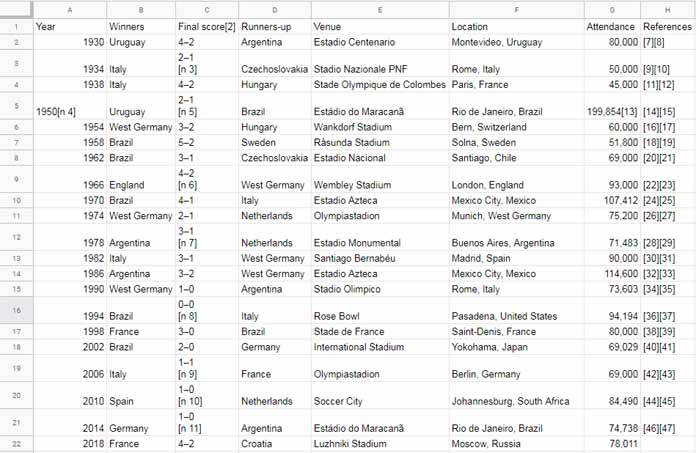
In this data what we want to concentrate is on the second column. The first column contains the year of the matches and the second column the names of the
Here I am going to use a Query formula. With the help of the Group By clause, you can count the values (country names) in column B. That will show the number of titles won by each nation.
=query(B1:B22,"Select B, count(B) where B is not null group by B",1)Screenshot # 5:
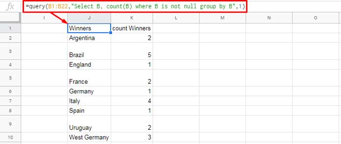
In this summary, you can see the winners and count, I mean the result by the nation. We have not used the Order By clause in Query to sort the data. The Group By clause automatically sorted the country names alphabetically.
Here comes the importance of my workaround and see that result first.
Screenshot # 6:
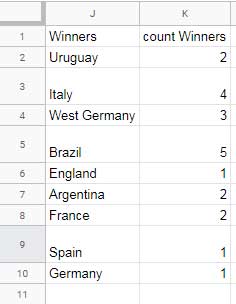
In this example, I have applied my workaround to avoid auto sorting in the Query Group By clause. So the output keeps the original order of the source data.
In this particular source data (screenshot # 4), column A contains years of the FIFA World Cup final matches.
Keeping the original order of column B in the summary (screenshot # 6) helps us to retain the winners (country) name by chronological order.
Workaround to Retain the Source Data Order in The Query Group By Clause
Here is the step by step instructions. Actually, the workaround to avoid auto sorting when using Query Group By clause involves four main functions – ROW, SORT, SORTN, and INDEX.
We want to group the range B2:B28 using Query (please refer to screenshot # 4).
Step # 1: Add a Sequential Number Column with the Grouping Column
This is the key. The below formula will add sequential numbers (2, 3, 4…) with the data in the range B2
=ArrayFormula({B2:B22,row(B2:B22)})Screenshot # 7:
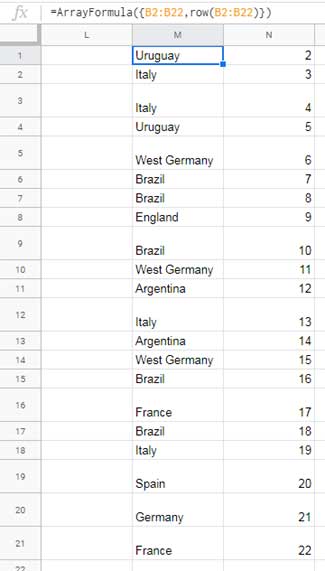
Under Step # 3, I’ve explained why we require this sequential number column.
Step # 2: Sorting of Grouping Column and Sequential Number Column
We must sort the column 1 in the above output in ascending order then by column 2 that also in ascending order.
So I am going to use the function SORT here. When using SORT, we can remove the ArrayFormula. See the generic formula first.
SORT({range}, sort_column, is_ascending, sort_column2,is_ascending2)Formula in line with the above generic formula.
=sort({B2:B22,row(B2:B22)},1,1,2,1)Step # 3: SORTN to Create a Single Row for Each Distinct Combination of Values
Now it’s time to use my one of the favorite function after Query. That’s none other than the SORTN.
You can use SORTN to remove the duplicates in column 1. In other words, similar to Query grouping, it creates a single row for each distinct combination of values.
The SORTN contains display tie mode numbers and the number # 2 in that is exclusively for removing duplicates.
SORTN(range, [n], [display_ties_mode], [sort_column], [is_ascending])The SORT formula under Step # 2 is the range in the SORTN. Here is that SORTN formula.
=sortn(sort({B2:B22,row(B2:B22)},1,1,2,1),9^9,2,1,1)[n] – the number of rows to return after removing the duplicates. We want the total rows after removing the duplicate rows. But we don’t know the exact number. So I’ve used 9^9 to represent “ALL”.
If you apply the below formula you can understand it.
=9^9Result: 387420489
2 – This after the [n] is the tie mode number to delete duplicates.
1 – The column to consider duplicates. It’s the column 1 that contain the country name.
1 – Ascending order. This sort order is very important. The Query group by clause sorts the grouping column in ascending order. So in SORTN also we must sort this column accordingly.
The SORTN formula returns the country names after removing duplicates in ascending order. It also contains the serial numbers as the second column.
See the screenshot in Step # 4 below. This serial number I will use later to Sort the Query output. That’s why I have told you earlier, it’s the key.
Step # 4: Extract the Sequential Number Column
Enter the below Query formula in cell J1 and the just above SORTN formula in cell M2 and compare the country names in each output. You can see that both are in the
=query(B1:B22,"Select B, count(B) where B is not null group by B",1)Screenshot # 8:
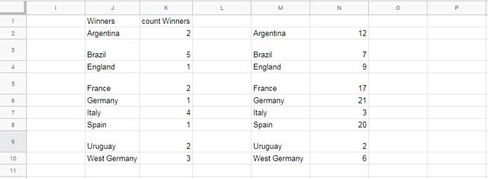
We only want the second column in the SORTN output. Using Index function we can offset the first column.
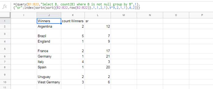
={"sr";index(sortn(sort({B2:B22,row(B2:B22)},1,1,2,1),9^9,2,1,1),0,2)}Additionally I have added a label “Sr” on the top (refer cell L1 on the screenshot # 9 below).
Step # 5: Prepare the Data to Avoid Auto Sorting When Using Query Group By Clause
Combine the Query formula and the above Index combo using Curly Brackets.
={query(B1:B22,"Select B, count(B) where B is not null group by B",1),{"sr";index(sortn(sort({B2:B22,row(B2:B22)},1,1,2,1),9^9,2,1,1),0,2)}}Screenshot # 9:
Step # 6: Final Step
In this final step, use the above three columns as the data in another Query and use the Order By clause to sort the third column in ascending order. Then extract column 1 and 2 only.
=Query({query(B1:B22,"Select B, count(B) where B is not null group by B",1),{"sr";index(sortn(sort({B2:B22,row(B2:B22)},1,1,2,1),9^9,2,1,1),0,2)}},"Select Col1,Col2 order by Col3 Asc")That’s all. This is the workaround to avoid auto sorting in Query Group By clause in Sheets.
Can I do the same with
Yes! The formula is almost the same.
=Query({query(B2:C8,"Select B, sum(C) group by B label sum(C)''"),index(sortn(sort({B2:B8,row(B2:B8)},1,1,2,1),9^9,2,1,1),0,2)},"Select Col1, Col2 order by Col3 asc")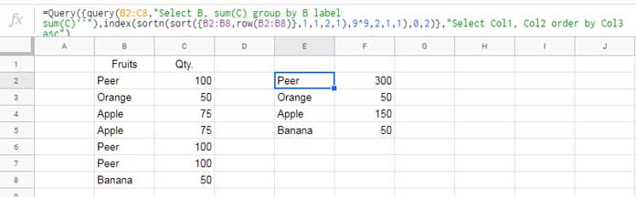
Thanks for the stay! Enjoy!