


We can use the Countif function to count across columns row by row in Google Sheets. But not as an array formula. So what is the alternative solution?
We can use MMULT as explained here in this tutorial How to Expand Count Results in Google Sheets Like Array Formula Does or the DCOUNT database function.
Also, we can now use a Lambda solution (New!) for the same.
If you use my MMULT, slightly modify it to incorporate the criteria that you want. I am not detailing that here.
I have been exploring the database functions in the last few tutorials, and here is one more. I’ve also included a simple solution using the new BYROW Lambda helper function.
Introduction
As far as I know, we can’t use the Countif function to count across columns row by row in Google Sheets.
In a non-array formula, the said function use will be as follows.
Problem:-
How to count the test scores which are greater than or equal to 10 (>=10), across columns in each row in Google Sheets?
Here we can use the below Countif formula in cell F2 and copy-paste (or drag the cell F2 fill handle using the mouse) down.
=countif(A2:E2,">=10")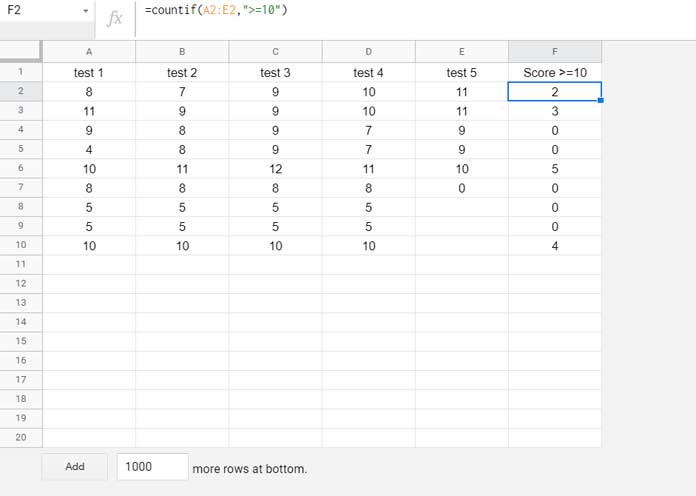
It will be tough to manage the above formula if you have several rows in your sheet with values to count.
When you insert new rows, each time, you may require to copy-paste the formula.
Hence, an array formula equivalent to Countif across columns row by row will be preferable.
As I have mentioned, we can use MMULT, DCOUNT, or a Lambda helper function for the same. This post explains the DCOUNT and Lambda use.
Countif Across Columns Row by Row Using DCOUNT in Google Sheets
Please note! Here, Countif means conditional count, not the function itself.
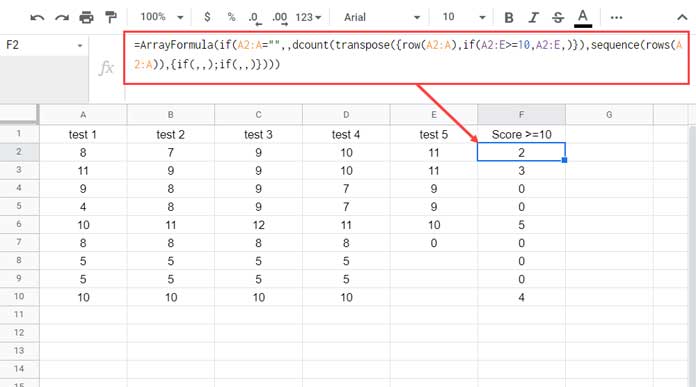
Array formula in cell F2 for the above same database:
=ArrayFormula(if(A2:A="",,dcount(transpose({row(A2:A),if(A2:E>=10,A2:E,)}),sequence(rows(A2:A)),{if(,,);if(,,)})))Note:-
1. If any cells in column A are blank, the formula will return nil.
So, if you see no count in any cell in column F, make sure that you have not left the corresponding cell in column A blank.
2. Only include the numeric value range.
I know database functions require a criteria column and a header row (field labels). With workarounds, we can exclude using them.
I have adopted the same in the above DCOUNT formula. I will explain them later.
The above is the array formula to Countif across columns row by row in Google Sheets.
DCOUNT Logic Used
DCOUNT Syntax: DCOUNT(database, field, criteria)
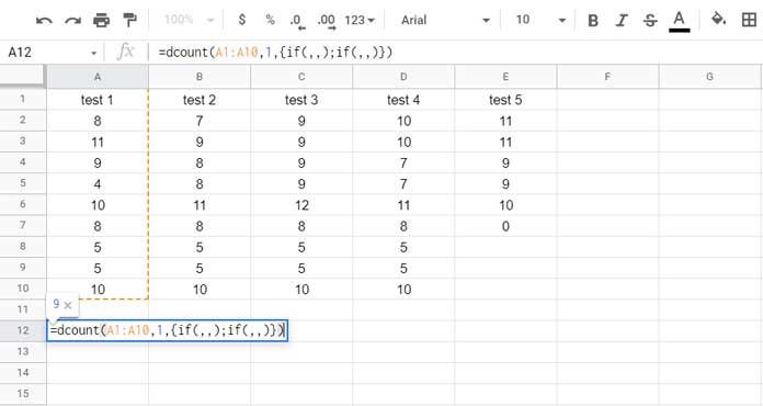
We can use DCOUNT as below to conditional count the values in a column.
=dcount(A1:A10,1,{if(,,);if(,,)})Please note, here I am talking about a column, not a row. We can, later on, come back to row.
I don’t want to specify any criterion. So in the formula, I have used {if(,,);if(,,)} which is equal to selecting two adjacent blank cells vertically.
To count multiple columns (columns A, B, C, D, and E) using DCOUNT, use ArrayFormula and change the reference in the formula accordingly. Also include all the field numbers as an array.
=ArrayFormula(dcount(A1:E10,{1,2,3,4,5},{if(,,);if(,,)}))To count the values in each column conditionally, for example, values >=10, we should change A1:E10 with if(A1:E10>=10,A1:E10,).
Here are the formula and output.
=ArrayFormula(dcount(if(A1:E10>=10,A1:E10,),{1,2,3,4,5},{if(,,);if(,,)}))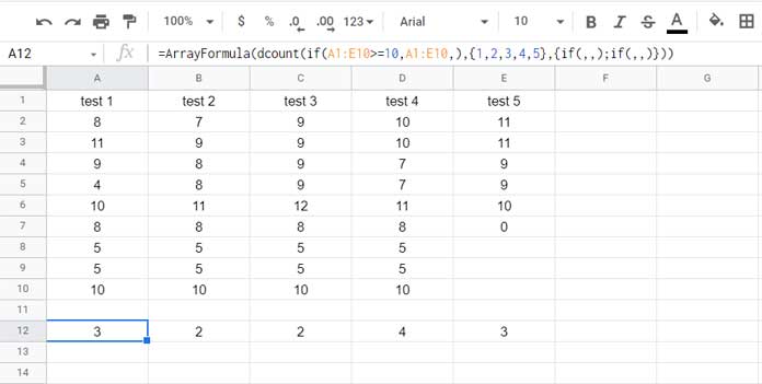
If you understand this conditional column count, you can effortlessly grasp how to Countif across columns row by row using DCOUNT in Google Sheets.
Because we just need to Transpose the range A2:E10 (not A1:E10).
Since we exclude the field labels in A1:E1, we must use virtual field labels for the formula to work correctly.
Please find those details below.
Formula Explanation
Please scroll to the top, and once again see the array formula to Countif across columns row by row in Google Sheets.
I am talking about the formula in cell F2. You can alternatively refer to the below image.
The arguments in use as per the DCOUNT syntax are as follows.
Database
transpose({row(A2:A),if(A2:E>=10,A2:E,)})When we transpose (change the data orientation) the range A2:E10, there won’t be any field labels. But using them is a must in DCOUNT.
So, I have populated the row numbers of A2:A and combined them with the range if(A2:E>=10,A2:E,).
Once transposed, it (the row numbers) will act as the field labels of if(A2:E>=10,A2:E,).
Field
sequence(rows(A2:A))What we are doing is Countif across columns row by row in Google Sheets.
For that, we have transposed the data and returned the count of columns of the transposed data vertically, not horizontally.
That will be equal to the conditional count row by row.
The above Sequence formula returns the field numbers from 1 to n vertically by counting total rows in the range A2:A.
Criteria
{if(,,);if(,,)}We have no criteria column to specify. So used the above formula to return two blank cells.
Other Formula Parts
if(A2:A="",,Outside the DCOUNT, I have used the above IF test.
It is because we have infinite rows in our database. This logical test helps us to return the result only in the rows where column A has values.
That’s all about how to use DCOUNT to conditional count across columns and return row-by-row output in Google Sheets.
Countif Across Columns Row by Row Using the BYROW Function (New)
We can now expand a COUNTIF formula to conditionally count values across columns row by row using BYROW in Google Sheets.
You may key in the below BYROW formula in cell F2.
=byrow(A2:E,lambda(r,if(counta(r)=0,,countif(r,">="&10))))It will populate values in F2:F, provided cells in F3:F blank.
Can you explain this formula to us?
Why not? Here you go!
Base Non-Array Formula:
=countif(A2:E2,">=10")Array Formula Using BYROW Lambda Formula:
=byrow(A2:E,lambda(r,countif(r,">=10")))The above formula returns 0 in blank rows. To return blank, we have additionally used if(counta(r)=0,,
Thanks for the stay. Enjoy!
Hi, That works great. Those lambda functions are fantastic.
Many thanks for sharing!
Thanks for this.
What would the formula look like if you wanted to compare (row by row) against the values in a column?
I.e., not a fixed value like 10, but, e.g., 8 for the first row in the table, 9 for the second, etc.
Hi, Steve,
Please see if this formula help.
=byrow(ArrayFormula(if(A2:E>=F2:F,A2:E,)),lambda(r,count(r)))It compares A2:E against F2:F and returns the count.