This is the first time I took lots of time to properly title a post. Still, I’m unsure whether I’ve justified to the tutorial below. Also, I can’t call it a tutorial. I am going to provide you with a Custom Formula to Use for Start Date and End Date Based Calculations in Google Sheets. What type of calculations?

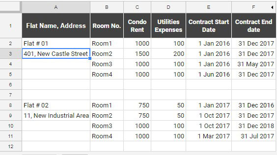
You can use the logical test part of the formula to check the start and end dates for your purpose. I will come to that later. Now, first of all, please check the below image and understand the sample data.

What I am going to do here is calculating the revenue for a certain period. For example, for Room 1, the monthly condo rent is 1000 and utility expense is 100. That means total income from the rental is 1100 monthly. I am not mentioning the currency as it’s not important for our purpose here.

There are four rooms in Flat # 01. What will be my total income from these rooms for a certain period? For example, I want to generate a report where the report start date is 1 Jan 2015 and end date is 30 Jun 2016. Here I should get the rental for all the rooms during that period but be considering the start and end date of the contract.

So I have a formula for you for this purpose. Let us understand the above concept with little more details.

Start Date and End Date Based Calculations in Google Sheets

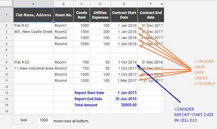
On the image, I’ve marked what the formula will consider based on the report start and end date provided.

Don’t get? See the contract start date and contract end date on the image above. It’s from 01 Jan 2016 to 31 Dec 2017 for Flat # 01 and different dates for Flat # 02. But we require the Condo Rent + Utility expense for the period from 1 Jan 2015 to 30 Jun 2016 (report start and report end date).

It’s not possible as the report start date here contradicts with the contract start date. So here the formula should consider the Contract Start Date except in one case where the contract start date is 1 October 2014. Here the formula should consider Report Start Date, i.e., 1 Jan 2015 as we want to run the report from this date.

The same condition is applicable to Report End Date and Contract End Date also. Here I’ve added one more logical test that if the contract end date is Nil, the formula should consider the current date as contract end date. So I have a foolproof logical test here.

Hope you understood the concept. You can’t probably do it with FILTER, QUERY, SUMPRODUCT or SUMIFS functions. We should either use IF or IFS logical functions for this purpose.

So I made a logical formula using nested IF, that will check all the above date related aspects and do the calculation. You can use the same formula for logical tests related to the start and end date and change the calculation part based on your requirement. Also, I have used some date functions on the calculation part you can learn that Here.

The calculation part I’ve highlighted below for the first logical test and that is applicable to rest of the logical tests in the same formula. You can use the logical test part for your purpose and modify the calculation part. The calculation part is just simple. We have the monthly rental on the above data. I calculated the per day rental and then used that to calculate the total rental for the Report Start and Report End Date period.

In cell G2, I’ve applied the below formula, then copied and pasted it to adjoining cells down.

=round(iferror(IF(and(E2<MASTER!$E$13,MASTER!$E$13<>"",F2<>"",F2>MASTER!$E$14),((C2+D2)*12/365*(datedif(MASTER!$E$13,MASTER!$E$14,"D")+1)),
IF(and(E2<MASTER!$E$13,MASTER!$E$13<>"",F2<>"",E2<>"",F2<=MASTER!$E$14),((C2+D2)*12/365*(datedif(MASTER!$E$13,F2,"D")+1)),
IF(and(E2>=MASTER!$E$13,MASTER!$E$13<>"",F2<>"",E2<>"",F2>MASTER!$E$14),((C2+D2)*12/365*(datedif(E2,MASTER!$E$14,"D")+1)),
IF(and(E2>=MASTER!$E$13,MASTER!$E$13<>"",F2<>"",E2<>"",F2<=MASTER!$E$14),((C2+D2)*12/365*(datedif(E2,F2,"D")+1)),
IF(and(E2>=MASTER!$E$13,MASTER!$E$13<>"",F2="",E2<>"",today()<=MASTER!$E$14),((C2+D2)*12/365*(datedif(E2,today(),"D")+1)),
IF(and(E2>=MASTER!$E$13,MASTER!$E$13<>"",F2="",E2<>"",today()>MASTER!$E$14),((C2+D2)*12/365*(datedif(E2,MASTER!$E$14,"D")+1)),
IF(and(E2<MASTER!$E$13,MASTER!$E$13<>"",F2="",E2<>"",today()<=MASTER!$E$14),((C2+D2)*12/365*(datedif(MASTER!$E$13,today(),"D")+1)),
IF(and(E2<MASTER!$E$13,MASTER!$E$13<>"",F2="",E2<>"",today()>MASTER!$E$14),((C2+D2)*12/365*(datedif(MASTER!$E$13,MASTER!$E$14,"D")+1)),0)))))))),"0"),0)

Here is the Sample Sheet Where I did these calculations.

Sample Spreadsheet [Please make a copy of this sheet and use]. If you find this custom formula useful, please drop in comments.