


This post describes how to use the XLOOKUP function in visible data in Google Sheets. We will use a Lambda LHF with the SUBTOTAL for this.
We can temporarily hide unwanted or unused data in cells in 2-3 ways in Google Sheets. What are they?
We usually use Data > Create a filter or Data > Filter view > Create a new filter view.
I’m sure you are familiar with that method. There are other methods and here are them.
- View > Group > Group row.
- Right-click on a select row(s) and hide that row(s).
XLOOKUP has many options to lookup a range. But there is no option to exclude hidden rows.
To XLOOKUP visible data, we require to use one other function, i.e., SUBTOTAL.
But the drawback is it’s not an array formula that spills down in rows. So we may additionally require to use the BYROW or MAP LHFs.
That will help us to expand/spill down a SUBTOTAL result.
I prefer the former function to add the spill capability to the SUBTOTAL function.
How to XLOOKUP Visible Data in Google Sheets
XLOOKUP has plenty of options to customize searching a key/value in search mode and match mode. I’m not detailing that since it’s already explained within the relevant tutorial.
Here we will use a basic formula to learn XLOOKUP in visible data in Google Sheets. You may have additional questions that you can post in the comment below.
Sample Data (Un-filtered)
We have the codes of a few items in column A and corresponding quantities in column B. I haven’t filtered the data currently.
In this data, to get the quantity of the first item ending with 1003, we can use a wildcard match in XLOOKUP as follows.
=XLOOKUP("*1003",A2:A,B2:B,"Not Available!",2,1)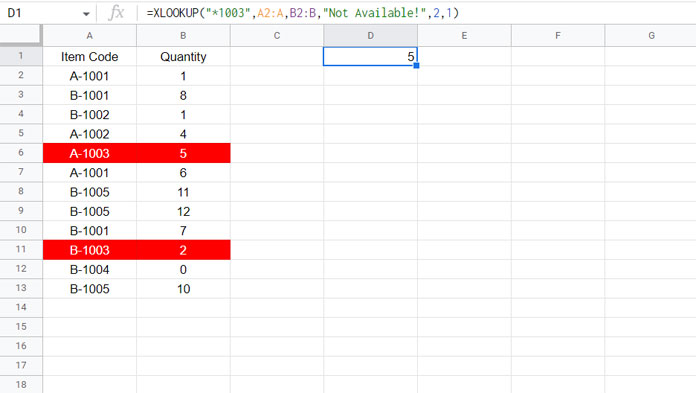
Syntax:
XLOOKUP(search_key, lookup_range, result_range, [missing_value], [match_mode], [search_mode])search_key: *1003
lookup_range: A2:A
result_range: B2:B
missing_value: Not Available!
match_mode: 2 (wildcard match)
search_mode: 1 (from first value to last value)
Now let’s see how the above XLOOKUP works in visible or filtered data in Google Sheets.
Sample Data (Filtered) and XLOOKUP in Visible Data
First, I’m filtering A1:B using Data > Create a filter. Then Filter column A by the following custom formula in Filter by condition.
=not(regexmatch(A2,"A"))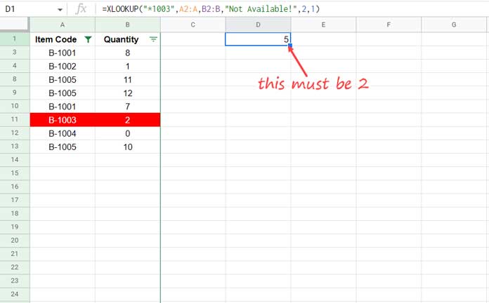
As you can see, the XLOOKUP formula in cell D1 is not excluding hidden rows. It returns the value in the hidden row.
To XLOOKUP visible data, please do as follows.
We can use the following BYROW formula to find filtered data in Google Sheets.
=BYROW(A2:A,LAMBDA(range,SUBTOTAL(103,range)))Note:- Please check BYROW (function guide) for the formula explanation.
It will return either 1 or 0 in A2:A, depending on the status of the rows, i.e., hidden or not.
The BYROW and SUBTOTAL combination formula will return 1 in all non-blank visible rows and 0 in all hidden rows.
Logic:
By adding 1 to the search_key and the above formula to lookup_range (the last part of both), we can exclude hidden rows in XLOOKUP.
Sometimes, the number 1 may already be a part of your search_key. To avoid that issue, instead of 1, add “^1” and make the same change in the lookup_range.
Since we combine two arrays (adding a BYROW array result to the lookup_range), we must use the ArrayFormula with the XLOOKUP.
Here is the formula for XLOOKUP visible (filtered) data in Google Sheets.
=ArrayFormula(xlookup("*1003^1",A2:A&"^"&BYROW(A2:A,LAMBDA(range,SUBTOTAL(103,range))),B2:B,"Not Available",2,1))That’s all. Thanks for the stay. Enjoy!