


This tutorial explains how to use the WRAPROWS function in Google Sheets. A similar function is already available in Excel, so some of you might be acquainted with it.
Google introduced a slew of new functions in early 2023, and WRAPROWS is among them, mostly falling under the “Array” category.
What is the purpose of the WRAPROWS function in Google Sheets?
We use the text wrapping (Format > Wrapping > Wrap) command to wrap text within a cell.
However, prior to the introduction of WRAPROWS, there was no specific command or function to wrap a provided row or column of values, necessitating reliance on workarounds.
Related: How to Move Each Set of Rows to Columns in Google Sheets
This is where the WRAPROWS and WRAPCOLS functions prove beneficial. How do these two functions differ?
The former function wraps the provided row or column of cells by rows, whereas the latter does so by columns.
Note:
The function is already featured in the Google Docs help center article here.
If the formula in this tutorial returns a #NAME?, it indicates that the WRAPROWS function has not been made available in your Sheets as of now. Please await the completion of the rollout.
Syntax and Arguments
Syntax: WRAPROWS(range, wrap_count, [pad_with])
Arguments:
range: The range to wrap (a single row or column).
wrap_count: A number representing the maximum number of cells for each row in the output.
If wrap_count isn’t a whole number (e.g., 4.8), the function will round it down to the nearest whole number (4 here).
pad_with: An optional argument in the WRAPROWS function.
If you omit this argument, the function will fill the extra cell(s) with #N/A. For example, if there are seven elements and the wrap_count is 4, the formula will return #N/A in the eighth cell.
Examples of the Use of the WRAPROWS Function in Google Sheets
It’s not too difficult to understand the WRAPROWS function in Google Sheets. Here are a few examples.
Considering there are ten elements in the vertical range A2:A11, let’s wrap it by rows using the WRAPROWS function in Google Sheets.
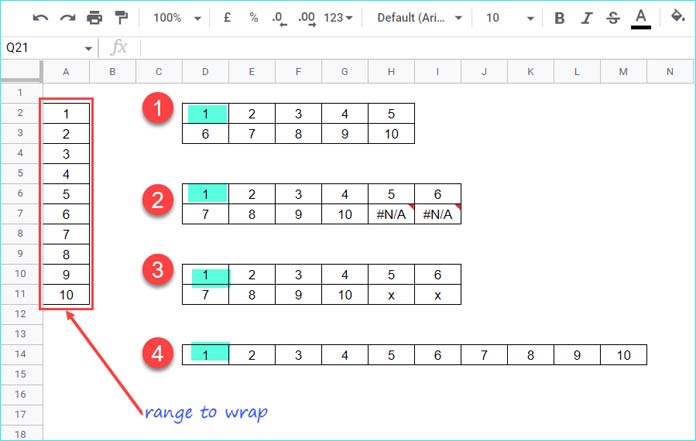
1. Maximum 5 Numbers Per Each Row:
=WRAPROWS(A2:A11, 5)2. Maximum 6 Numbers Per Each Row:
=WRAPROWS(A2:A11, 6)The formula returns two #N/A errors since the total elements in the range are 10, not 12.
3. Replacing #N/A Errors in the WRAPROWS Function:
=WRAPROWS(A2:A11, 6, "x")4. Matching Total Elements in the Range and Wrap Count:
=WRAPROWS(A2:A11, 10)The formula will return the same range.
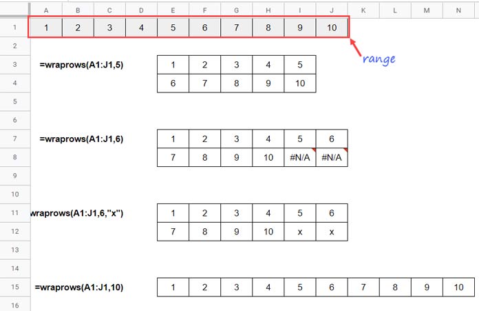
What happens when we have a horizontal range?
The following screenshot is self-explanatory.
WRAPROWS Function and Unstacking of Data (Real-life Use)
In a previous tutorial, we explored the process of unstacking data in Google Sheets.
Typically, we work with stacked data due to the exemplary ease it provides for data manipulation.
However, unstacked data is generally more reader-friendly.
For basic unstacking, the WRAPROWS function in Google Sheets comes in handy. Here’s an example:
Let’s assume you have a category column in A and a value column in B. You can unstack this data if each category contains the same number of rows.
Here is one approach to unstack such data in Google Sheets:
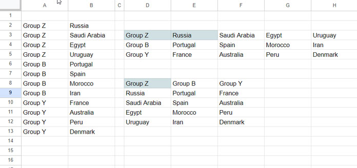
Here, each category contains 4 rows. So the wrap_count in the WRAPROWS formula will be 4.
In cell E3:
=WRAPROWS(B2:B13, 4)In cell D3 (Supporting UNIQUE Formula):
=UNIQUE(A2:A13)Now, for the formula in D8:
The above two formulas return a table with a horizontal layout where headers appear in the first column of the table.
To easily transpose the orientation, we need to stack the results of the two formulas horizontally and then transpose it.
Here is the formula for achieving this:
=TRANSPOSE(HSTACK(UNIQUE(A2:A13), WRAPROWS(B2:B13, 4)))
Dear Prashanth,
Thank you very much for your blog, which is a great inspiration and an excellent source for finding answers regarding the creative and effective use of Google Sheet functions.
Regarding this article, especially the last section about using WRAPROWS to unstack:
I am a little confused about the screenshot.
With UNIQUE of columns A, we would determine the number of categories, i.e., the number of columns in the resulting table.
At the same time, the number of elements per category is different. It seems like the wrapping creates an offset of 1 per row (3 vs. 4).
Have a great day!
Hi John Edward,
Thanks for pointing out the issue. I’ve replaced the screenshot and modified the formulas accordingly.
Have a great day too!