The VLOOKUP function in Google Sheets searches all rows in the first column of the search range, irrespective of whether the rows are hidden or visible. However, sometimes you may want the VLOOKUP function to skip hidden rows when searching for a key in Google Sheets. In such cases, you should use a helper column with VLOOKUP.
The purpose of the helper column is to verify whether a row is hidden or not. We can create the helper column using the SUBTOTAL function, which works only with visible rows.
Preparing the Helper Column for VLOOKUP in Visible Rows Only
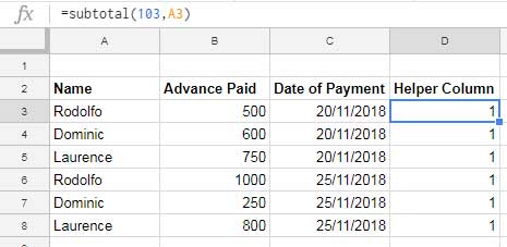
Assume you have sample data in A2:C8 with the columns Name, Advance Paid, and Date of Payment. You can use the range D2:D8 as the helper column.
In cell D3 (leaving the first row for headers), use the following SUBTOTAL formula and drag it down to cell D8:
=SUBTOTAL(103, A3)This formula returns 1 for rows that are visible and 0 for hidden rows.

If you prefer not to use a drag-down formula, you can convert it into a custom LAMBDA function and use it with a MAP helper function to iterate through each row in the range.
To replace D3:D8, insert the following formula in cell D3:
=MAP(A3:A8, LAMBDA(val, SUBTOTAL(103, val)))The MAP helper function applies the custom LAMBDA function (LAMBDA(val, SUBTOTAL(103, val))) to each row in the range A3:A8.
Notes:
You can replace 103 in the formula with 3. Both represent COUNTA, but 103 skips all hidden rows, whereas 3 skips only rows hidden via filtering (e.g., using a Data Filter or Slicer).
The SUBTOTAL reference must be from the first row of the search column, i.e., the very first cell in the range.
Formula Example: VLOOKUP Skips Hidden Rows in Google Sheets
Example Data
- Range: A3:C8 (excluding hedder row)
- Search Key: Dominic (from the first column)
- Index Column: 2 (Column B, the formula will return a value from this column).
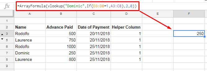
The name “Dominic” is in cells A4 and A7. If row 4 is hidden, the following regular VLOOKUP formula would still return the value 600, which is in the hidden cell B4:
=VLOOKUP("Dominic", A3:C8, 2, 0)Correct VLOOKUP Formula to Skip Hidden Rows
To skip hidden rows, use the following formula:
=ARRAYFORMULA(VLOOKUP("Dominic", IF(D3:D8=1, A3:C8), 2, 0))
Explanation of the Formula
The helper column plays a vital role in the formula. Instead of directly using A3:C8 as the VLOOKUP range, the formula uses a logical IF statement referencing the helper column. Here’s the modified range:
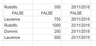
IF(D3:D8=1, A3:C8)This range excludes rows where D3:D8 equals 0 (hidden rows). To make this work across the entire range, you must wrap the formula in ArrayFormula:
=ARRAYFORMULA(IF(D3:D8=1, A3:C8))Output:

Visible rows in the lookup range remain intact, while hidden rows are replaced with FALSE values. This ensures the VLOOKUP search key does not match any hidden rows.
Additional Resources
- Calculate the Average of Visible Rows in Google Sheets
- IMPORTRANGE to Import Visible Rows in Google Sheets
- XLOOKUP Visible (Filtered) Data in Google Sheets
- XMATCH Visible Rows in Google Sheets
- Weighted Average of Filtered (Visible) Data in Google Sheets
- UNIQUE Function in Visible Rows in Google Sheets
- SUMIF Excluding Hidden Rows in Google Sheets
- How to Exclude Hidden Rows in Google Sheets QUERY
- COUNTIF | COUNTIFS Excluding Hidden Rows in Google Sheets


