


In this tutorial, let’s learn to make a vertical line graph in Google Sheets. I’m using a workaround method that only supports a single line (series).
Vertical line charts are not commonly used to represent data graphically. So obviously, that might be the reason for no such chart option built into Google Sheets.
Line Graphs are the best way to visualize how the quantity/value of something changes over time.
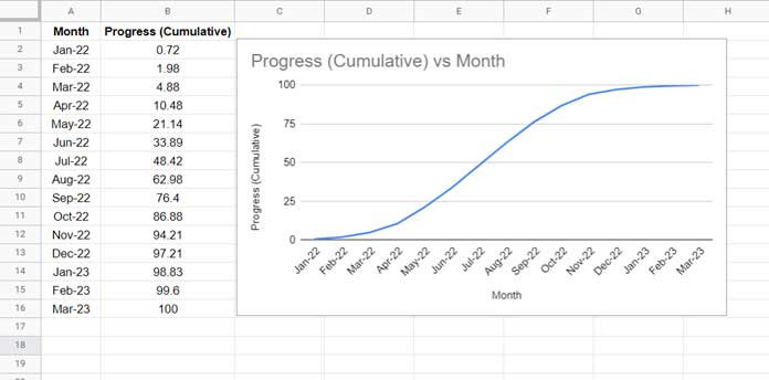
Sample Data:-
(Please feel free to skip the explanation below)
For example, we can plot such a chart to show how your work progress over time (view data by month).
Regarding representing work progress by month graphically, we can visualize either a month-wise or a cumulative month-wise data using a line chart.
How do they differ?
- Using monthly progress data, we can see month-wise progress over time.
- If you use the running total of monthly progress data, you will get the cumulative progress over time.
Below we will make a vertical line graph to visualize project progress over 15 months. The values are cumulative. So we will get cumulative progress over time.
Here is the sample data and the standard chart. Let’s see how to make a vertical line graph using the same data.
You May Like: How to Create S Curve in Google Sheets and Its Purpose in Scheduling.
Making Single Line Vertical Line Graph in Google Sheets
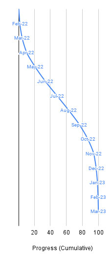
The line in the vertical line graph will look like the 90° CW rotated line in the above standard chart.
The vertical axis will be the horizontal axis, but the axis line will be at the bottom instead of on the top.
The category (horizontal) axis will be missing. Labels replace them in the vertical line chart in Google Sheets. Here it is.
Data Formatting – Category Axis, Data Points, and Labels
First of all, let’s try to understand the data to plot the vertical line graph.
Category Axis: C2:C16
In the first standard chart, the source data is in the cell range A2:B16, whereas in the second vertical one, it’s in A2:C16 because we have used a helper range additionally.
It’s an array formula in cell C1, which populates backward sequential numbers. Here is that formula.
={"Helper";sequence(15,1,15,-1)}The SEQUENCE function returns 15 numbers (we have data points in 15 rows in B2:B16) in descending order, such as C1 = “Helper,” C2 = 15, C3 = 14, C4 = 13, and so on.
Data Points: B2:B16
It’s the cumulative progress over time. We can use these values as it is.
Labels: A2:A16
It is the category axis in the standard line chart. Here in the vertical line graph, we will use them as labels.
You must format them to “Plain Text” by highlighting A2:A16 and applying Format > Number > Plain Text.
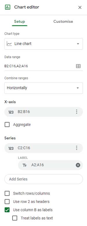
Steps to Make Vertical Line Chart in Google Sheets
Let’s make the vertical line graph in Google Sheets now.
- Select B2:C16.
- Apply Insert > Chart. It will insert a chart into your sheet, and the chart editor panel will also be opened.
- There are two tabs within the chart editor panel – Setup and Customize. Under the first tab, make sure you have the following essential settings to plot the vertical line chart.
| Chart Type | Line Chart |
| X-axis | B2:B16 |
| Series | C2:C16 |
| * Labels | A2:A16 |
* Click on the three vertical dots next to the series C2:C16 and select “Add labels.”
Google Sheets will add labels that may or may not be correct.
We want to add labels from A2:A16. If not getting it, edit the just added one.
The vertical line graph is almost ready. What is left is the customization of the chart. Go to the concerned tab within the chart editor.
Go through each option and make the necessary changes. Here are a few of them.
Chart and axis titles > Chart title > Title text – Empty it.
Chart and axis titles > Vertical axis title – Title text – Empty it.
That’s all. Thanks for the stay. Enjoy!
Related Chart Resources
- How to Create a Bell Curve Graph in Google Sheets.
- Depreciation Curves in Google Sheets – How to and Sample Sheet.
- How to Create a Candlestick Chart in Google Sheets.
- Sparkline Line Chart Formula Options in Google Sheets.
- Scatter Chart in Google Sheets and Its Difference with Line Chart.
- How to Plot a Line Chart Using Lap Times in Milliseconds in Google Sheets.
- Create a Shaded Target Range in a Line Chart in Google Sheets.