


If you use varying array sizes in a Countifs formula in Google Sheets, you will get an error. It’s because the function doesn’t support such usage.
It usually happens when you specify mismatching columns in criteria range 1 and 2 in Countifs.
You may please go through the function syntax first. It’s as follows.
Syntax: COUNTIFS(criteria_range1, criterion1, [criteria_range2, …], [criterion2, …])
When you specify multiple criteria ranges, all the arrays/ranges should have the same size vertically and horizontally.
That means the number of rows and columns should match or be the same in all the specified criteria ranges/arrays.
Let’s quickly go to an example to understand it.
=countifs(A2:D10,"Apple",E2:E10,"Yes")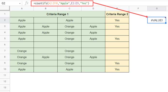
Here are the four arguments in use.
1. criteria_range1 – A2:D10
2. criterion1 – “Apple”
3. criteria_range2 – E2:E10
4. criterion2 – “Yes”
As you can see, the above two array arguments (criteria_range1 and criteria_range2) to COUNTIFS are different in size.
There are four columns in the first array (argument 1) and one column in the second array (argument 3).
In the above example, I want to count the “Apple” in multiple column range A2:D10 if the values in E2:E10=”Yes.”
Workarounds to Use Varying Array Sizes in Countifs in Google Sheets
I have three workaround formulas for you to try when you have varying array sizes in Countifs that cause the #VALUE! as above.
I may be able to come up with more. But the below options will be sufficient for you.
Option 1 – Varying Array Sizes in Countifs with Virtual Criteria Ranges
We can follow different approaches to use varying array sizes in Countifs in Google Sheets.
To logically fit the Countifs rule, we can create a virtual criteria_range2 with an equal number of columns.
We have earlier adopted this method in SUMIF, i.e., to return the Sum of Matrix Rows or Columns Using Sumif in Google Sheets.
I am following the same technique with COUNTIFS here.
Formula # 1:
=countifs(A2:D10,"Apple", ARRAYFORMULA(if(E2:E10="Yes",column(A2:D2)^0)),1)Result: 9
The above is the first option to specify mismatching columns in criteria range 1 and 2 in Countifs.
Want to learn the above COUNTIFS formula in detail?
Formula Explanation
criteria_range1 – A2:D10
criterion1 – “Apple”
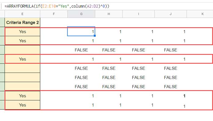
criteria_range2 – ARRAYFORMULA(if(E2:E10="Yes",column(A2:D2)^0))
criterion2 – 1
In the Countifs (Formula # 1), the criteria_range2 is an array formula.
It would return an array with the number of columns equal to the criteria_range1.
The number of rows is already equal in both arrays, i.e., in criteria_range1 and 2.
This virtual array will have the number 1 in each column corresponding to “Yes” in E2:E10. That’s why I have used # 1 instead of “Yes” in criterion_2.
Here are the other two options that you can consider over the above formula.
Option 2 – Based on Filtering and Logical Tests
Without virtually matching varying array sizes in Countifs, we can get our desired result.
You can find below two such formula combinations, and I have marked my recommended formula also.
Formula # 2 (Recommended):
=countif(flatten(filter(A2:D10,E2:E10="Yes")),"Apple")Here I have used Countif instead of Countifs as we have only one column after manipulating the data with FILTER and FLATTEN.
It works like this.
- The Filter filters the rows in the range A2:D10 if E2:E10 is “Yes.”
- The Flatten makes four columns into one column.
- The Countif does the rest (counts the “Apple”).
Formula # 3:
=sum(ArrayFormula(if((A2:D10="Apple")*(E2:E10="Yes")=1,1,)))The above is another formula to consider when we have varying array sizes to specify in Countifs in Google Sheets.
How does this formula return the count of values conditionally from multiple mismatching columns?
Here is how!
The logical test, the formula enclosed within SUM, returns the # 1 wherever both conditions match. Please see the below illustration.
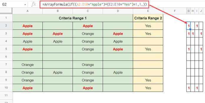
The SUM function returns the sum of those values.
If you have doubts about the array formula that I have used within SUM, you can learn that here – How to Use IF, AND, OR in Array in Google Sheets.
It’s just an alternative way to code AND logical test in array form.
I hope you could understand the above tips.
Thanks for the stay. Enjoy!
Countif | Countifs Resources
- Countifs with Multiple Criteria in the Same Range in Google Sheets.
- Countif in an Array in Google Sheets Using Vlookup and Query Combo.
- How to Use COUNTIF with UNIQUE in Google Sheets.
- Countif | Countifs Excluding Hidden Rows in Google Sheets.
- Google Sheets: Countifs with Not Equal to in Infinite Ranges.
- COUNTIFS in a Time Range in Google Sheets [Date and Time Column].
- COUNTIF to Count by Month in a Date Range in Google Sheets.
- Not Blank as a Condition in Countifs in Google Sheets.