


")


")

")
")
 in Excel & Google Sheets")


Using OFFSET with XLOOKUP and XMATCH, you can easily perform a two-way lookup and return multiple columns in Google Sheets. Here, “multiple columns” refers to all columns from the intersection point across the range.
For example, you can search for a fruit name in the first column of a range and a month name across the first row, then return the quantity of that fruit for the given month and all subsequent months.
Generic Formula
=OFFSET(XLOOKUP(A10, column, data), 0, XMATCH(A11, row)-1)Where:
columnis the first column in the data.rowis the first row in the data.A10contains the search key for the column.A11contains the search key for the row.
Let’s apply this two-way lookup formula in a real-life scenario to return multiple columns of data.
Example: Two-Way Lookup and Returning Multiple Columns in Google Sheets
In the following example, we have student names in column A, dates in row 1, and the attendance status (present/absent) of each student in the corresponding cells.
We’ll apply a two-way lookup to search for a student in the first column and a specific date in the first row, then return their attendance data from that point onward.
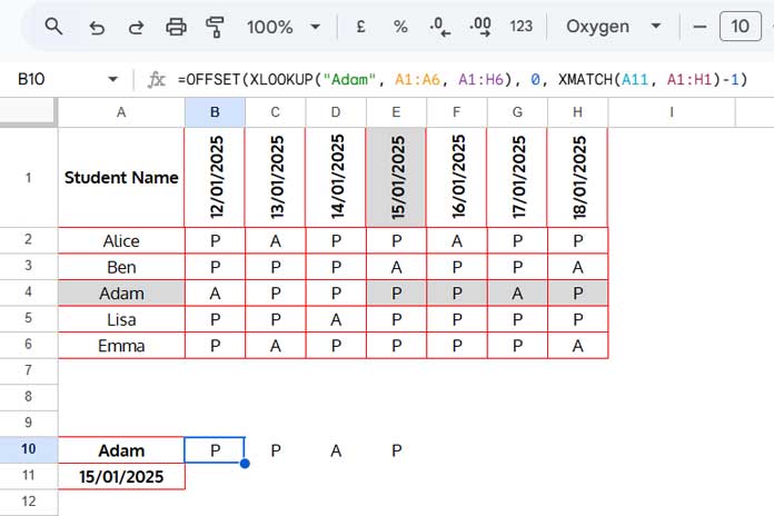
This method helps extract the attendance of a specific student from a given date onward, making it useful for analyzing a portion of the dataset.
Formula:
=OFFSET(XLOOKUP("Adam", A1:A6, A1:H6), 0, XMATCH(A11, A1:H1)-1)The formula searches for “Adam” in A1:A6 and the date in A11 within the first row, then returns the attendance records from that point onward.
Formula Breakdown
This formula is essentially an OFFSET function:
OFFSET(cell_reference, offset_rows, offset_columns, [height], [width])Where:
- cell_reference:
XLOOKUP("Adam", A1:A6, A1:H6)– Finds the row corresponding to “Adam”. - offset_rows:
0– Keeps the lookup on the same row. - offset_columns:
XMATCH(A11, A1:H1)-1– Determines the column offset by matching the date in the header row. Subtracting 1 aligns it with the 0-based index system used by OFFSET.
Alternative Solution: Two-Way Lookup to Return Multiple Columns
You can replace XLOOKUP with INDEX-MATCH and XMATCH with MATCH as an alternative.
Alternative Formula:
=OFFSET(INDEX(A1:H6, MATCH(A10, A1:A6, 0)), 0, MATCH(A11, A1:H1, 0)-1)Where:
- cell_reference:
INDEX(A1:H6, MATCH(A10, A1:A6, 0))– The MATCH function locates “Adam” in the first column, and INDEX retrieves the corresponding row. - offset_rows:
0– No row offset. - offset_columns:
MATCH(A11, A1:H1, 0)-1– Finds the column position of the date.
Additional Tip: Two-Way Lookup and Return Two Columns
The above formulas return all the columns after the intersection point of the two search keys. However, sometimes you may only need to return two columns.
For example, in an employee dataset similar to the one above, instead of just present and absent statuses, you might have an overtime column after each date as well.
In such cases, the purpose of the two-way lookup and returning multiple column values will be limited to two columns.
You can achieve this by specifying the width argument in the OFFSET function.
First Formula:
=OFFSET(XLOOKUP("Adam", A1:A6, A1:H6), 0, XMATCH(A11, A1:H1)-1, 1, 2)Second Formula:
=OFFSET(INDEX(A1:H6, MATCH(A10, A1:A6, 0)), 0, MATCH(A11, A1:H1, 0)-1, 1, 2)Can We Use VLOOKUP in This Case?
No, VLOOKUP cannot be used within OFFSET because it does not return a direct cell reference.
Resources
- How to Perform Two-Way Lookup Using VLOOKUP in Google Sheets
- Two-Way Lookup with XLOOKUP in Google Sheets
- Replace VLOOKUP and HLOOKUP with MATCH and INDIRECT in Google Sheets
- XLOOKUP and Offset Results in Google Sheets
- Slicing Data with XLOOKUP in Google Sheets
- Two-Way Filter in Google Sheets: Vertical & Horizontal
- Nested XLOOKUP Function in Google Sheets
What would be the formula to do a 2-way Lookup and Sumproduct the inside i.e. multiple June values for the “banana”?
Hi, Jamie Chung,
Why don’t you wrap the formula with Sumproduct? Both solutions would work in that way.
Eg.:
=sumproduct(OFFSET(index(B2:N6,match(F9,B2:B6,0)),0,match(F10,B2:N2,0)-1))