You can dynamically isolate specific subsets of data from a larger dataset, a process known as slicing data, using the XLOOKUP function in Google Sheets.

Typically, we use functions such as FILTER and QUERY for slicing data based on multiple criteria, such as date range, product category, price range, or customer location.

Here is a scenario where you can’t use these functions to filter the data without the support of additional functions.

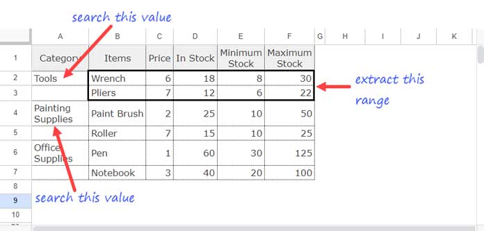
In this table, how do you filter the items that fall under the “Tools” category?

Two items fall under the said category: “Wrench” and “Pliers”. To improve readability, the category name is not repeated in the first column, making criteria-based filtering difficult.

This highlights the importance of data slicing using XLOOKUP.

Here is an XLOOKUP hack where we will extract specific data ranges by lookup. This method uses two XLOOKUP functions with the colon (:) range operator in between.

Vertical Data Slicing Using XLOOKUP in Google Sheets

Our sample data is in A1:F, and A1:F1 contains the following field labels:

Category | Items | Price | In Stock | Minimum Stock | Maximum Stock

Assume I want to look up the category column and slice the data from “Items” to “Maximum Stock.” The objective is to extract data related to the Tools category.

Below you will find the step-by-step instructions to extract data dynamically using XLOOKUP in Google Sheets. But first, here is the syntax of the function for your quick reference:

XLOOKUP(search_key, lookup_range, result_range, [missing_value], [match_mode], [search_mode])

Step-by-Step Explanation

1. Starting Point of the Range:

XLOOKUP("Tools", A2:A, B2:B)

This formula searches for “Tools” in A2:A and returns the corresponding value from B2:B. This will return the starting point of the range to slice.

2. End Point of the Range:

XLOOKUP("Painting Supplies", A2:A, F2:F)

This formula searches for “Painting Supplies” in A2:A and returns the corresponding value from F2:F. This will return the end point of the range to slice.

Key Points:

• The lookup_range in both formulas can be any column.
• The result_range controls the slicing start and end points.

Dynamic Range Formula:

To convert this to a dynamic range, place the colon operator in between the two XLOOKUP functions:

=XLOOKUP("Tools", A2:A, B2:B):XLOOKUP("Painting Supplies", A2:A, F2:F)

This will slice the data from the first lookup value to the last lookup value.

Adjusting the End Point:

If you don’t want the last row, use OFFSET with the end point (second XLOOKUP) to offset 1 row backward:

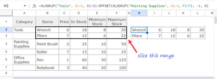
=XLOOKUP("Tools", A2:A, B2:B):OFFSET(XLOOKUP("Painting Supplies", A2:A, F2:F), -1, 0)

In this formula, the OFFSET function follows the syntax OFFSET(cell_reference, offset_rows, offset_columns, [height], [width]), where offset_rows is -1 and offset_columns is 0.

This way, we can dynamically slice data using XLOOKUP in Google Sheets.

Horizontal Data Slicing Using XLOOKUP in Google Sheets

You can apply this XLOOKUP hack in a horizontal lookup as well.

For example purposes, I’ve transposed the above sample data, and the range is 1:6.

Here is the formula that slices the range as earlier:

=XLOOKUP("Tools", 1:1, 2:2):OFFSET(XLOOKUP("Painting Supplies", 1:1, 6:6), 0, -1)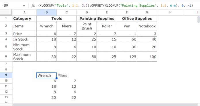

Explanation

1. Starting Point of the Range:

XLOOKUP("Tools", 1:1, 2:2)

The first XLOOKUP searches for the key “Tools” in the first row and returns the corresponding value from the second row, which is the starting point of the slicing range.

2. End Point of the Range:

XLOOKUP("Painting Supplies", 1:1, 6:6)

In the second XLOOKUP, the search_key is “Painting Supplies.” It searches in the first row and returns the value from the sixth row, which is the end point of the slicing range.

3. Adjusting the End Point:

OFFSET(XLOOKUP("Painting Supplies", 1:1, 6:6), 0, -1)

This time the OFFSET function offsets 0 rows and 1 column backward.

This technique provides a powerful way to dynamically slice and extract specific data ranges in Google Sheets. This data-slicing method can leverage advanced lookup capabilities to slice data accordingly.

Resources

Here are some other XLOOKUP resources:

• XLOOKUP Visible (Filtered) Data in Google Sheets
• XLOOKUP Nth Match Value in Google Sheets
• Nested XLOOKUP Function in Google Sheets
• XLOOKUP with Multiple Criteria in Google Sheets
• XLOOKUP for Multiple Column Results in Google Sheets
• XLOOKUP with Date and Time in Google Sheets
• XLOOKUP with Single IMPORTRANGE & LET in Google Sheets
• XLOOKUP and Offset Results in Google Sheets
• XLOOKUP in Merged Cells in Google Sheets
• Counting XLOOKUP Results with COUNTIFS in Excel and Google Sheets
• SUMIFS with XLOOKUP in Excel and Google Sheets