You can replace the VLOOKUP and HLOOKUP functions with a combination of MATCH and INDIRECT in Google Sheets. This approach offers several advantages:
- You can specify the column letter in vertical lookup instead of the column number from which you want to return the result.
- You can extract values to the left, right, bottom, and top of the lookup value.
- You can extract a 2D array from the lookup point.
The main drawback of this approach compared to traditional VLOOKUP/HLOOKUP is its inability to search for multiple search keys at once. Another drawback is that this approach may seem a little complex at first, but once you become familiar with it, you’ll find it easy to use.
Here are examples of transforming the MATCH function into VLOOKUP and HLOOKUP using INDIRECT.
Replacing VLOOKUP with MATCH and INDIRECT Combo in Google Sheets
Let’s consider the following sample data in B2:D12, which contains ranks, countries/regions, and apple production data for 2022:
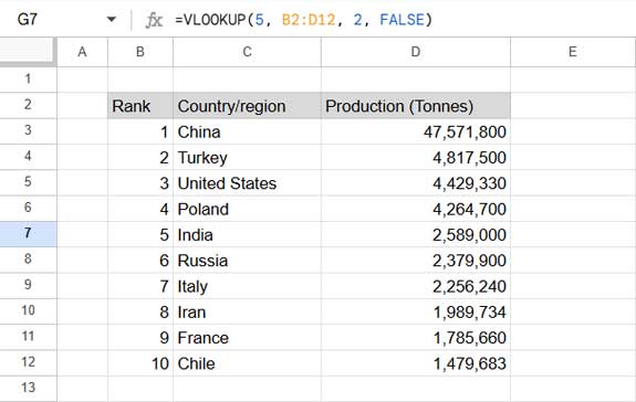
Assume you want to look up the country holding the fifth rank in apple production. Normally, you would use the following VLOOKUP formula:
=VLOOKUP(5, B3:D12, 2, FALSE) // returns "India"This formula searches for the rank 5 in the first column of the range and returns the corresponding country name from the second column.
Here’s how you can replace this VLOOKUP with the MATCH and INDIRECT combo:
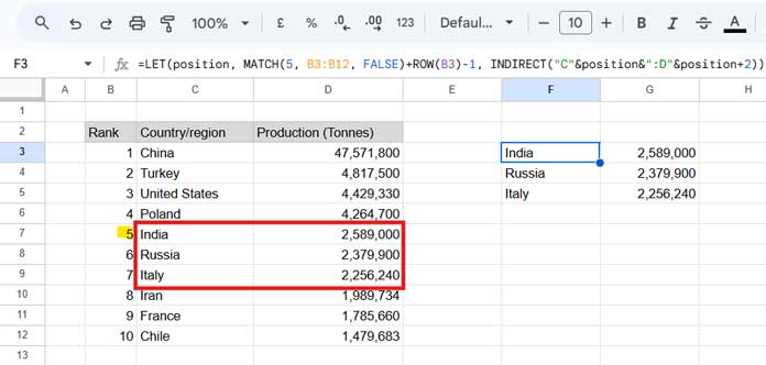
=LET(position, MATCH(5, B3:B12, FALSE)+ROW(B3)-1, INDIRECT("C"&position)) // returns "India"MATCH(5, B3:B12, FALSE)finds the rank5in the rangeB3:B12and returns its relative position.ROW(B3)-1adjusts for the row number above the range used inMATCH.- The sum of these gives the row number of the lookup value, assigned to the variable “position.”
INDIRECT("C"&position)retrieves the value from columnCat thepositionrow.
Why This Formula Matters
As mentioned earlier, this formula allows you to retrieve values from the left, right, top, bottom, and even return 2D results. Here are some examples to help you understand the full potential:
INDIRECT("C"&position-1)– gets the country (Poland) from the row immediately above.INDIRECT("C"&position+1)– gets the country (Russia) from the row immediately below.INDIRECT("D"&position)– retrieves the apple production value (2,589,000) from column D.INDIRECT("C"&position&":C"&position+2)– returns the country and the next two countries (India, Russia, and Italy).INDIRECT("C"&position&":D"&position+2)– retrieves the country and its production, along with the next two countries and their production.
With these variations, you can easily manipulate the INDIRECT portion of the formula to get values from various positions relative to the lookup value.
Replacing HLOOKUP with MATCH and INDIRECT Combo in Google Sheets
The approach to replacing HLOOKUP with MATCH and INDIRECT differs slightly. Here, data is arranged horizontally, and the ranks, country names, and production quantities are in rows 2, 3, and 4, respectively. The range is B2:L4.
The following HLOOKUP formula searches for rank 5 in the first row of the range and returns the country name from the second row:
=HLOOKUP(5, B2:L4, 2, FALSE)Here’s how you can replace this HLOOKUP with the MATCH and INDIRECT combo:
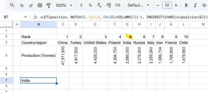
=LET(position, MATCH(5, C2:L2, FALSE)+COLUMN(C2)-1, INDIRECT(CHAR(64+position)&3))MATCH(5, C2:L2, FALSE)matches rank 5 in the range C2:L2 and returns the relative position of the column.COLUMN(C2) - 1adjusts for the number of columns before the range.- When you add the second value to the first, you get the actual column number of the lookup value, referred to as “position.”
CHAR(64 + position)converts the column number to its corresponding letter (e.g., for column 7, it will return “G”).CHAR(64 + position) & 3returns the cell address of the lookup value.INDIRECT(...)retrieves the value from the third row in the specified column.
Adjusting with INDIRECT
Here are some examples of how to adjust rows or columns using the INDIRECT formula:
Adjust Rows:
INDIRECT(CHAR(64 + position) & 3 & ":" & CHAR(64 + position) & 4) – returns the third and fourth rows from the column.
Adjust Columns:
INDIRECT(CHAR(64 + position - 1) & 3)– returns the value from the left of the lookup value from the third row.INDIRECT(CHAR(64 + position + 1) & 3)– returns the value from the right of the lookup value from the third row.INDIRECT(CHAR(64 + position) & 3 & ":" & CHAR(64 + position + 1) & 4)– returns the value from the third and fourth rows from the lookup column and the next column.
With these adjustments, you can transform the MATCH function to replace HLOOKUP in Google Sheets.


