In a Google Sheets file, I have a column contain text and numbers. I want to use Sumif in that text and number column in Google Sheets.
Naturally, the Sumif function won’t work in such data types. We must format the data first. Let me elaborate on how to format data for Sumif in this case.
Normally we enter text in one column and number in another column so that we can Sum or Sumif the number column. But here the scenario is different.
For example, see the below values in cell A1, A2, and A3.
Scenario 1 (Table 1):
| Sunday 25 |
| Monday 30 + Tuesday 40 |
| Tuesday 20 |
I want to sum the Total of “Tuesday” which would be 60. That’s what I meant to say Sumif in a text and number column in Google Sheets.
There is one more scenario that may be more common in real life. Here, there would be a number column too (A1:B3).
The value in the number column (column B) must be ignored if there are numbers in the text column in the corresponding row (example row # 2).
Scenario 2 (Table 2):
| Sunday | 25 |
| Monday 30 + Tuesday 40 | 70 |
| Tuesday | 20 |
Let’s see how to use Sumif function in these types of text and number column in Google Sheets.
How to Use SUMIF Formula in a Text and Number Column in Google Sheets
The first priority here must go to data formatting, not to the Sumif formula.
I am starting with scenario 1. Here are the steps to use Sumif in a text and number column in Google Sheets.
SUMIF Single Column Text and Number Values in Google Sheets
This is, of course, a step by step approach. If I give you the final Sumif formula now, you won’t probably understand that. So let me write the formula from scratch.
1. Remove ‘+’ Sign Using Regexreplace
Use the following Regexreplace in cell B1 to Remove the ‘+’ sign from the values. This sign separates one text and number from another.
=ArrayFormula(regexreplace(A1:A,"\+",""))Needless to say, if the separator is different change it accordingly in the above formula. If there is no separator, skip the above step.
2. TextJoin to Combine Sumif Range
This is the second step to use SUMIF in a text and number column in Google Sheets.
We can TextJoin the above Regexreplace output or if you have skipped step 1 simply use A1:A. The formula in cell B1 will be as follows.
=textjoin("",1,ArrayFormula(regexreplace(A1:A,"\+","")))
OR
=textjoin("",1,A1:A)
I know, at this juncture, you may want to see the output. Here you go!
Sunday 25Monday 30 Tuesday 40Tuesday 20I’ll use the TextJoin and Regexreplace combo formula for my examples below.
3. Split Numbers and Text to Use in Sumif as Range and Sum Range
Keeping the above Sumif problem in mind, I mean Sumif text and number in Google Sheets, I’ve recently written a Regex tutorial – How to Split Number from Text When No Delimiter Present in Google Sheets.
We can apply the formula mentioned in that guide/tutorial here to split the value in cell B1.
I mean we can split numbers from text and with some workaround, then use it as range and sum range in a Sumif formula.
In cell C1, you can see the formula explained in my above-mentioned guide.
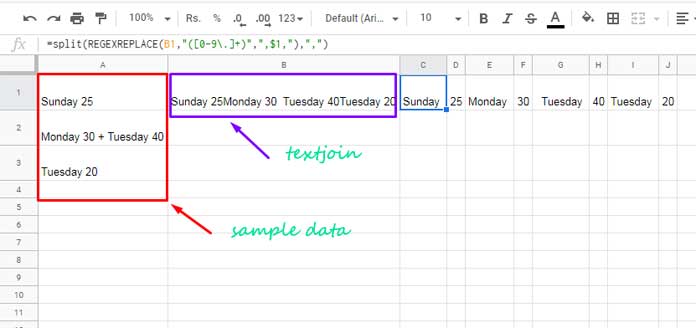
In that formula replace B1 with the Textjoin formula from B1. So that we can make cell B1 empty. Here is that formula.
=split(REGEXREPLACE(textjoin("",1,ArrayFormula(regexreplace(A1:A,"\+",""))),"([0-9\.]+)",",$1,"),",")Then transpose (change orientation) it. To do that, simply wrap the formula with the Transpose function.
=transpose(split(REGEXREPLACE(textjoin("",1,ArrayFormula(regexreplace(A1:A,"\+",""))),"([0-9\.]+)",",$1,"),","))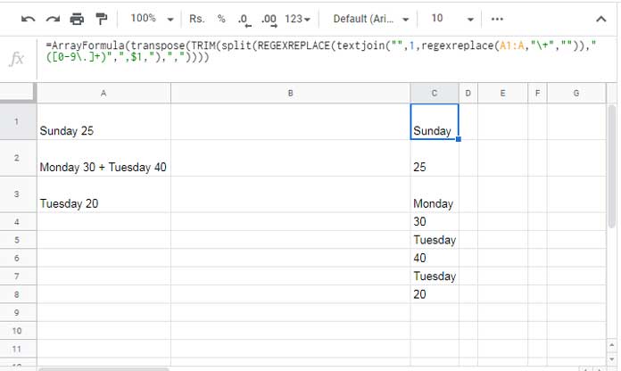
4. Move Text and Numbers to Separate Column Using Filter
We have reached the final step to use SUMIF in a text and number column in Google Sheets.
Actually we can use the following Filter formulas to filter text to one column and numbers to another column.
Filter Texts (E1):
=filter(trim(C1:C8),istext(C1:C8))Replace the range/array C1:C8 with the formula from cell C1. So the above formula will be;
=filter(trim(transpose(split(REGEXREPLACE(textjoin("",1,ArrayFormula(regexreplace(A1:A,"\+",""))),"([0-9\.]+)",",$1,"),","))),istext(transpose(split(REGEXREPLACE(textjoin("",1,ArrayFormula(regexreplace(A1:A,"\+",""))),"([0-9\.]+)",",$1,"),","))))Filter Numbers (F1):
=filter(C1:C8,isnumber(C1:C8))Here also replace the array C1:C8 with the formula from cell C1.
=filter(transpose(split(REGEXREPLACE(textjoin("",1,ArrayFormula(regexreplace(A1:A,"\+",""))),"([0-9\.]+)",",$1,"),",")),isnumber(transpose(split(REGEXREPLACE(textjoin("",1,ArrayFormula(regexreplace(A1:A,"\+",""))),"([0-9\.]+)",",$1,"),","))))In this new data, we can use the SUMIF as usual. Cool, right?
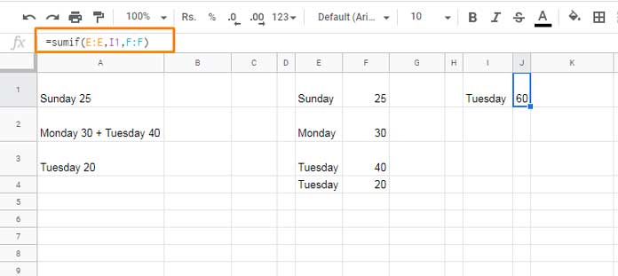
Multiple Column Text and Number and Sumif
Scroll up and see the second table. There are two columns. To use Sumif in such text and number columns in Google Sheets, we can’t use the above formula to format the data.
We must follow a few more additional steps in the beginning. Here are those steps.
1. Filter Text Contain Numbers
The below formula extracts texts which contain numbers (formula in cell C1).
=filter(A1:A,regexmatch(A1:A,"[0-9]+")=TRUE)Replace ‘+’ with a blank (please refer to the image below).
=regexreplace(filter(A1:A,regexmatch(A1:A,"[0-9]+")=TRUE),"\+","")2. Filter Text Doesn’t Contain Numbers
The opposite of the above formula in cell D1. This formula will return a two-column data.
=filter(A1:B,regexmatch(A1:A,"[0-9]+")=FALSE)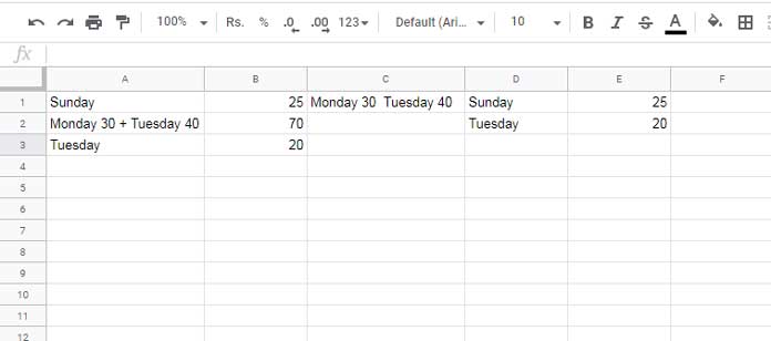
3. TextJoin Two Filters
Place the above two formulas inside a TextJoin as below.
=textjoin("",1,regexreplace(filter(A1:A,regexmatch(A1:A,"[0-9]+")=TRUE),"\+",""),filter(A1:B,regexmatch(A1:A,"[0-9]+")=FALSE))Output:
Monday 30 Tuesday 40Sunday25Tuesday20We are now ready to use SUMIF in a text and number column in Google Sheets. The rest of the steps are from point # 3 onwards under scenario 1.
You can skip those steps! How?
Just replace textjoin(“”,1,ArrayFormula(regexreplace(A1:A,”+”,””))) in scenario 1 final formulas in cell E1 and F1 with the just above (TextJoin two filters) formula.
So the formulas will be;
E1:
=filter(trim(transpose(split(REGEXREPLACE(textjoin("",1,regexreplace(filter(A1:A,regexmatch(A1:A,"[0-9]+")=TRUE),"\+",""),filter(A1:B,regexmatch(A1:A,"[0-9]+")=FALSE)),"([0-9\.]+)",",$1,"),","))),istext(transpose(split(REGEXREPLACE(textjoin("",1,regexreplace(filter(A1:A,regexmatch(A1:A,"[0-9]+")=TRUE),"\+",""),filter(A1:B,regexmatch(A1:A,"[0-9]+")=FALSE)),"([0-9\.]+)",",$1,"),","))))F1:
=filter(transpose(split(REGEXREPLACE(textjoin("",1,regexreplace(filter(A1:A,regexmatch(A1:A,"[0-9]+")=TRUE),"\+",""),filter(A1:B,regexmatch(A1:A,"[0-9]+")=FALSE)),"([0-9\.]+)",",$1,"),",")),isnumber(transpose(split(REGEXREPLACE(textjoin("",1,regexreplace(filter(A1:A,regexmatch(A1:A,"[0-9]+")=TRUE),"\+",""),filter(A1:B,regexmatch(A1:A,"[0-9]+")=FALSE)),"([0-9\.]+)",",$1,"),","))))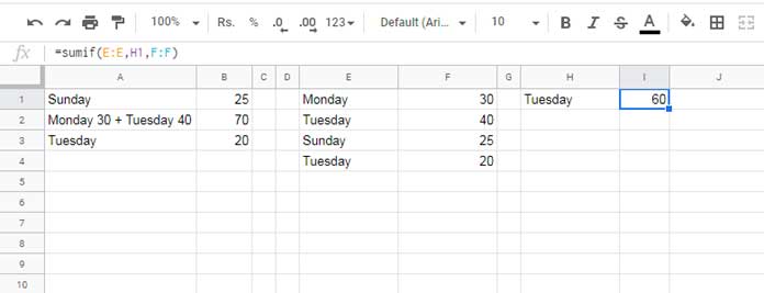
That’s all about using SUMIF formula in a text and number column in Google Sheets.
SUMIF Resources
- Sum by Month in Google Sheets Using Combined SUMIF Formula.
- How to Sum Every Nth Row in Google Sheets Using SUMIF.
- How to Sumif When Multiple Criteria in the Same Column in Google Sheets.
- Google Sheets SUMIF to Sum by Month and Year.
- SUMIF Formula to SUM Current Week’s Data in Google Sheets.
- How to Include Multiple Sum Columns in SUMIF in Google Sheets.
- SUMIF to Sum By Current Work Week in Google Sheets.
- Multiple Criteria Sumif Formula in Google Sheets.
- How to Sumif/Sumifs Excluding Duplicates in Google Sheets.
- Sumif Multiple Columns Criteria – It Works in Google Sheets.
- SUMIF Returns Multiple Columns in Google Sheets.
- Combined Use of Sumif with Vlookup in Google Sheets.
- Sumif Importrange in Google Sheets – Examples.


Hello
I have multiple columns where each cell is a number + currency in text or an EMPTY cell
eg:
50 USD
45 EUR
12 CHF
[EMPTY]
40 EUR
[EMPTY]
51 USD
Problem is that for these empty cells, the above formulae skip the empty cells and return value for the next cell that is not empty, breaking their correct order:
How do I keep the correct order of rows in each column?
Thanks!
Hi, Bojc,
I guess you just want to split the values. Assume your given values are in A1:A, then in B1 insert the following formula.
=ArrayFormula(IFERROR(split(A1:A," ")))Please see if that helps?