You can use the ampersand operator to concatenate columns and criteria, creating a multiple-criteria SUMIF formula in Google Sheets. The criteria can be from one column or two or more different columns. SUMIF supports multiple-column criteria this way in Google Sheets.
Why not use the SUMIFS function, which inherently supports multiple criteria, instead?
The reason is that the SUMIFS formula can’t expand; in other words, it returns a single-cell output.
Here, you will find the benefits of using SUMIF with multiple conditions in Google Sheets.
However, there are two shortfalls in using multiple criteria in SUMIF with the ampersand operator:
- It won’t work with comparison operators in SUMIF. For example, using a date difference as the condition in a SUMIF formula is not possible this way.
- You might not be able to use wildcards for partial matches.
Basic Example of SUMIF
Let me begin with the SUMIF syntax in Google Sheets:
SUMIF(range, criterion, [sum_range])Where:
rangeis the range to test against the criterion.criterionis the condition to test in the range.sum_rangeis the range to sum; it must be a physical range.
I know you are not new to SUMIF. Still, here is a basic example meant for those who are inexperienced in using the SUMIF function.
The sample data consists of fruit names in column A, countries of availability in column B, and yearly production in column C.

This single-criterion SUMIF formula sums column C if the value in column A is “Plum”.
=SUMIF(A1:A, "Plum", C1:C)There is no issue using multiple criteria in Google Sheets SUMIF within a single column. As an example, see how I use the SUMIF formula to sum the values of both “Plum” and “Apple”:
=ArrayFormula(SUMIF(A1:A, {"Plum", "Apple"}, C1:C)) // returns the result in two cellsWhen the criteria in SUMIF are in two different columns, you should either use the SUMIFS function or a combination formula with SUMIF.
Here is the ARRAYFORMULA + SUMIF + Ampersand combination.
How to Use Multiple Criteria in SUMIF in Google Sheets
We will see two examples here. The first one handles one criterion from each of two columns, and the second one handles three criteria, with one or more criteria from either column.
Example 1: One Criterion from Each Column
From our sample data, how do I get the sum of the total production of apples in the United States when the fruit names are in column A and the country names are in column B?
You can combine columns A and B and the criteria as shown in the example below:
=ArrayFormula(SUMIF(A1:A&B1:B, E2&F2, C1:C))
Note the use of the ARRAYFORMULA function because when we combine multiple values with the ampersand concatenation operation, it requires array support.
Also, use the criterion in cell references as above. Do not hardcode them like "AppleUnited States" instead of E2&F2 in the formula.
Hardcoding will strip off the advantage of multiple criteria SUMIF, which we will explore in the last part of this tutorial.
Example 2: One or More Criteria from Either Column
You’re about to learn a trick that nobody has told you about so far.
This is the tricky part of the multiple criteria SUMIF formula, which involves the SWITCH function as well.
Let’s assume you want to sum the total production quantity of apples and plums in the United States. How do you find that?
The criteria are entered in cells E2:G2, where E2, F2, and G2 contain “Apple”, “Plum”, and “United States” respectively.
SUMIF can’t handle this on its own by combining criterion and criteria columns. You can only use one criterion from each column. We can achieve this using the following logic:
Within the SUMIF, replace “Plum” in column A with “Apple” and use the criteria columns A2:A (the new virtual column) and B2:B, and the criterion E2&G2, not E2&F2&G2.
How do we do that?
We will use the SWITCH function to convert multiple criteria in a column into one criterion. Please see the highlighted part in the following SUMIF formula:
=ArrayFormula(SUMIF(SWITCH(A1:A, E2, E2, F2, E2, "")&B1:B, E2&G2, C1:C))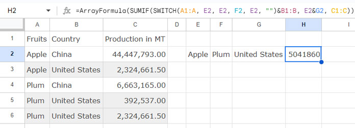
The SWITCH function follows the syntax SWITCH(expression, case1, value1, [case2, value2, …], [default]).
The expression to test is A1:A, and the cases to test are E2 (Apple) and F2 (Plum). We should use the value “Apple” (E2) to return in all cases. If there’s no match, the formula will return an empty string.
The Benefits of Using Multiple Criteria SUMIF Formula in Google Sheets
While we have the SUMIFS function specifically for multiple criteria usage, it has one drawback: it won’t expand the results into multiple rows without the help of the MAP lambda function.
The Lambdas may not work efficiently with very large datasets. Additionally, they can be a bit complex for newcomers to learn.
However, the SUMIF formulas can expand on their own if you simply combine criteria columns and criteria without using any other function to manipulate the criteria columns.
For example, we can adjust our example #1 formula to expand to two criteria rows as follows:
=ArrayFormula(SUMIF(A1:A&B1:B, E2:E3&F2:F3, C1:C))
However, this doesn’t apply to our example #2 formula, which involves the SWITCH function.
In that case, you can only use multiple country names in rows as per the example below:
=ArrayFormula(SUMIF(SWITCH(A1:A, E2, E2, F2, E2, "")&B1:B, E2&G2:G3, C1:C))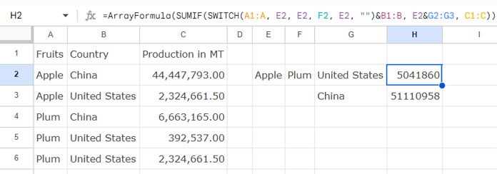
Resources
Here are some related resources.
- How to SUMIF When Multiple Criteria in the Same Column in Google Sheets
- Multiple Sum Columns in SUMIF in Google Sheets
- Dynamic Sum Column in SUMIF in Google Sheets
- How to Include Adjacent Blank Cells in SUMIF Range in Google Sheets
- Combined Use of SUMIF with Vlookup in Google Sheets
- SUMIF Importrange in Google Sheets – Examples
- Using SUMIF in a Text and Number Column in Google Sheets
- The Sum of Matrix Rows or Columns Using SUMIF in Google Sheets
- SUMIF with ArrayFormula in Filtered Data in Google Sheets
- How to Use the SUMIF Function Horizontally in Google Sheets
- SUMIF Across Multiple Sheets in Google Sheets
Hello,
I have two sheets I’m working with and having an issue with the Sheet1!B2 formula.
=ArrayFormula(SUMIFS(Sheet2!$B:$B,Sheet2!$C:$C,{"Indemnity - Property Damages"},Sheet2!$A:$A,A2))
This formula works by pulling data from Sheet 2.
I’m trying to combine the “Expense – Legal Coverage” and “Expense Legal Defense” into the criteria in the same formula in H2.
I have tried multiple ways and continually get errors.
Hi, Alex Shaw,
Thanks for giving edit access to your example sheet.
I’ve updated the formula in the test tab in your sheet as per this tutorial – SUMIFS with OR Condition in Google Sheets.
Hi, I’ve been trying to find a formula that works for what I need it to for a few days now, and I haven’t been successful.
All I’m trying to do is take the sum of 2 cells in the same column and make it highlight a certain color if their combined values equal 5, for example.
Is there such a formula for this?
Hi, Sam,
You may try this rule, please.
Cells: A4 and A6.
Apply to range (In conditional formatting):
A4,A6Format rule > Custom Formula (In conditional formatting):
=$A$4+$A$6=5