In this tutorial, you will receive a free monthly employee attendance sheet with formulas in Google Sheets. To use it effectively, follow the instructions provided in this tutorial.
The formulas are designed to summarize the leave categories you input for each employee under the respective days of the week. This feature enhances the attendance sheet, making it both distinctive and user-friendly.
Feel free to customize the template according to your preferences by adding row borders, titles, and other formatting elements. You can also replace the leave categories with those prevailing in your organization.
To access the template, click the button below.
Leave Categories and Customization
One of the specialties of my attendance sheet in Google Sheets is its flexibility in customization. Let’s begin with leave categories.
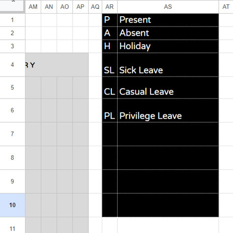
I’ve incorporated the following six common leave categories into my employee attendance sheet. Feel free to tailor them to align with your organization’s specific leave policies and categorizations.
- P: Present
- A: Absent
- H: Holiday
- SL: Sick Leave
- CL: Casual Leave
- PL: Privilege Leave
How do I modify the leave categories?
Navigate to column AR. You can customize the existing leave categories in AR1:AR10. Add more in the column or remove any as needed. The values in column AS are optional. A maximum of 10 leave types is supported.
Utilization of Leave Categories in the Attendance Template
We have implemented the above leave categories in four sections of the attendance sheet template: in the attendance area, in the summary area, to create a legend string, and within conditional formatting.
These settings do not require any adjustments. I provide this information to help you understand how to use the sheet for recording employee attendance.
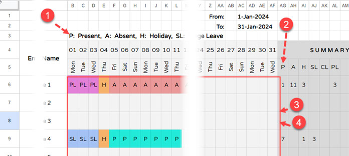
1. Legend String Formula in cell B3:
=TEXTJOIN(", ", TRUE, QUERY(TRANSPOSE(FILTER(HSTACK(AR1:AR10&": ", AS1:AS10), AR1:AR10<>"")),, 9^9))It generates the legend string “P: Present, A: Absent, H: Holiday, SL: Sick Leave, CL: Casual Leave, PL: Privilege Leave”. The formula is flexible and will adjust according to your entered leave categories in the AR1:AS10 range.
This is a somewhat complex formula and is optional. If you are interested in understanding it, I recommend reading about the TEXTJOIN function and the flexible join formula in QUERY.
2. Formula in Cell AG5 for Field Labels in AG5:AP5:
=TOROW(AR1:AR10, 1)This TOROW formula takes the range AR1:AR10, removes any empty cells, and arranges the non-empty values in a single row.
3. Drop-Downs in B6:AF100:
We used the categories in AR1:AR10 to create drop-downs in the B6:AF100 range, the attendance area in the sheet.
Instead of manually typing the leave type, double-click on any cell to select the leave type from a drop-down.
4. Highlighting in B6:AF100:
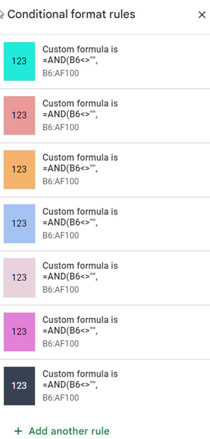
I’ve employed 10 custom formula rules to highlight each selected category in the range B6:AF100. If you are dissatisfied with the color selection, you can modify it.
Click on any cell in the range and navigate to Format > Conditional formatting. Select the rule you want to change the color for.
Four Essential Formulas for Creating an Attendance Sheet
We discussed two formulas above. They are optional and added for flexibility in the layout. You can manually enter the values returned by these formulas. This is not the case with the following formulas.
I’ve included four essential formulas in the free attendance sheet.
Formula #1:
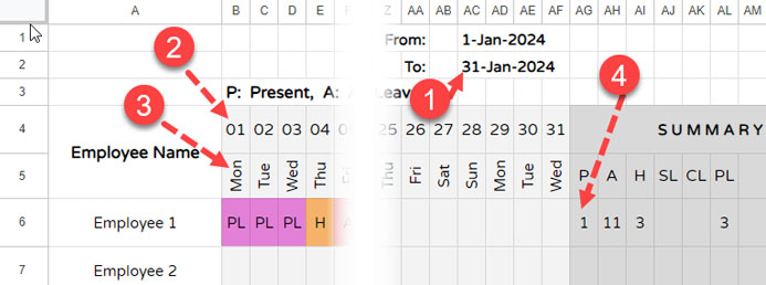
=EOMONTH(AC1, 0)Manually enter the month start date in cell AC1. This EOMONTH formula returns the end-of-month date in cell AC2.
Formula #2:
=SEQUENCE(1, AC2-AC1+1, AC1)This formula in cell B4 takes the start date in cell AC1 and the end date in cell AC2 to generate a sequence of dates during that period in the range B4:AF4.
- 1: Number of rows
- AC2-AC1+1: Number of columns
- AC1: Starting sequence from
Formula #3:
=ArrayFormula(IF(LEN(B4:AF4), TEXT(B4:AF4, "DDD"),))In cell B5, this formula returns the corresponding names of the days of the week in the range B5:AF5.
The TEXT function formats the data, and the LEN part excludes blank cells in the last columns based on the number of days in the month.
Formula #4:
=BYROW(B6:AF, LAMBDA(v, MAP(AG5:AP5, LAMBDA(r, LET(test, COUNTIF(v, r), IF(test=0, ,test))))))- This is the key formula that returns the summary of attendance categories in each row.
How to Utilize the Attendance Sheet Template
Simply enter the month’s start date in cell AC1, employee names in A6:A, and select attendance categories in B6:AF. The sheet will take care of the rest.
Resources
In this tutorial, you received a free attendance template and all the details to use it effectively. I’ve also provided brief descriptions of the formulas in use.
Additionally, we offer some other professional free templates. Here are a few of them.
- Dynamic Yearly Calendar Template in Google Sheets
- Fully Flexible Fiscal Year Calendar In Google Sheets
- Reservation and Booking Status Calendar Template in Google Sheets
- Calendar View in Google Sheets (Custom Template)
- Hourly Time Slot Booking Template in Google Sheets
- Create Gantt Chart Using Formulas in Google Sheets
- Array Formula to Split Group Expenses in Google Sheets
- Create a Habit Tracker in Google Sheets: Step-by-Step Guide