In Google Sheets, you might often need to search for a specific value across multiple columns and return the corresponding column header. This is particularly useful when you’re working with structured data, where categories are listed in headers and associated data is placed below them. For example, you may have multiple projects listed in the headers and machinery deployed under each project. In this case, you might want to search for a specific machinery type and return the project it is allocated to.

In this tutorial, you’ll learn three different formulas for searching across columns and returning matching headers. Each formula serves a different purpose:

1. A case-insensitive match formula.
2. A modified version of the first formula that allows partial matches.
3. A case-sensitive match formula for exact keyword matching.

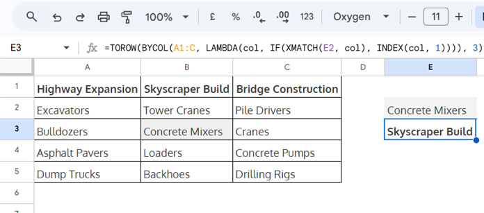
Below is a screenshot to show how the search across columns and return header works with Formula Approach 1.

Case-Insensitive Formula to Search Across Columns and Return the Header in Google Sheets

Consider the following data range: A1:C, where A1:C1 contains the project names (e.g., Highway Expansion, Skyscraper Build, Bridge Construction).

Let’s say you want to search for “Concrete Mixers” under these projects and return the project name(s). If the same machinery is deployed under multiple projects, you’ll want to return all matching project names.

Exact Match:

1. Enter the keyword “Concrete Mixers” in cell E2.
2. Enter the following formula in cell E3:

=TOROW(BYCOL(A1:C, LAMBDA(col, IF(XMATCH(E2, col), INDEX(col, 1)))), 3)

This formula is case-insensitive and searches across the columns to return the header in Google Sheets.

How Does This Formula Work?

• XMATCH(E2, col) checks for a match of the search key in the current column and returns the relative position if a match is found; otherwise, it returns #N/A.
• IF(.., INDEX(col, 1)) checks if the XMATCH function returns a number. If so, the INDEX function returns the first row of the current column (i.e., the header).
• BYCOL applies this logic to each column in the array, returning either the header or #N/A values.
• TOROW removes any error values, leaving only the matched headers.

Partial Match:

To allow for partial matching, you can modify the formula by using the wildcard * on both sides of the search key in XMATCH, and specifying match mode 2.

The updated formula will be:

=TOROW(BYCOL(A1:C, LAMBDA(col, IF(XMATCH("*"&E2&"*", col, 2), INDEX(col, 1)))), 3)

This will allow partial matches of the search key, and it’s still case-insensitive.

Simply enter “Mixers” in cell E2. The formula will locate “Concrete Mixers” in the columns and return the corresponding header.

Case-Sensitive Formula to Search Across Columns and Return the Header in Google Sheets

In some cases, case sensitivity is important, especially when you’re dealing with item codes, usernames, etc.

Using the same data set from above, here’s the formula to search for an exact case-sensitive match and return the headers:

=TOROW(BYCOL(A1:C, LAMBDA(col, INDEX(col, IF(SORTN(EXACT(col, E2), 1, 0, 1, 0), 1, -1)))), 3)

Formula Explanation:

• EXACT(col, E2) compares the search key with each value in the current column and returns an array of TRUE or FALSE values.
• SORTN(..., 1, 0, 1, 0) sorts the array in descending order, keeping the TRUE values at the top (if a match is found).
• IF(..., 1, -1) returns 1 if TRUE (indicating a match) and -1 if FALSE.
• INDEX(col, ...) returns the header of the current column if there’s a match, otherwise it returns #NUM error.
• BYCOL applies the formula to each column in the array and returns either the header or #NUM error.
• TOROW removes any errors, leaving only the valid headers.

This formula performs a case-sensitive search across columns and returns the corresponding headers.

Conclusion

By using these formulas, you can easily search across columns and return the header in Google Sheets. Whether you need an exact match, partial match, or case-sensitive match, these formulas provide flexible options for working with structured data in Sheets.

These techniques are especially useful when handling large datasets where manually searching for specific data could be time-consuming.

Related Resources:

• Lookup and Retrieve Column Headers in Google Sheets
• Find the Column Header of the Max Value in Google Sheets
• Find the Column Header of the Min Value in Google Sheets
• Find Max N Values in a Row and Return Headers in Google Sheets
• Get the Headers of the First Non-Blank Cell in Each Row in Google Sheets
• Get the Header of the Last Non-Blank Cell in a Row in Google Sheets