We often use the QUERY function to aggregate data in Google Sheets, and the GROUP BY clause helps with this. However, when using this clause, only aggregated values are returned, omitting individual row details. Fortunately, there is a way to retain all values in QUERY GROUP BY—by adding a helper column to your source data.
This tutorial will show you how to structure your data and formula to retain all values within each group, ensuring you don’t lose important row-level details.
Sample Data and Regular Aggregation with Missing Row-Level Data
Assume you have the following sales data in A1:C:
| Category | Item | Sales (kg) |
| Fruits | Rambutan | 12.5 |
| Fruits | Blueberry | 8.2 |
| Fruits | Orange | 20 |
| Vegetables | Carrot | 15.4 |
| Vegetables | Tomato | 18.7 |
| Vegetables | Spinach | 9.3 |
| Vegetables | Spinach | 7.8 |
To get a category-wise summary, you can use the following QUERY formula:
=QUERY(A1:C, "select A, sum(C) where A is not null group by A", 1)Result:
| Category | sum Sales (kg) |
| Fruits | 40.7 |
| Vegetables | 51.2 |
The formula selects and groups column A (Category) and totals column C (Sales). Since we used an open range (A1:C), we opted to filter out empty rows in the data to ensure a clean result.
Here, the row-level data is missing because the ‘Item’ column is omitted. We want to include the Item column as well, but without grouping it.
However, every column used in the SELECT clause must also be included in the GROUP BY clause. This means the following formula will not work:
=QUERY(A1:C, "select A, B, sum(C) where A is not null group by A", 1)Example of Retaining All Values When Using QUERY GROUP BY
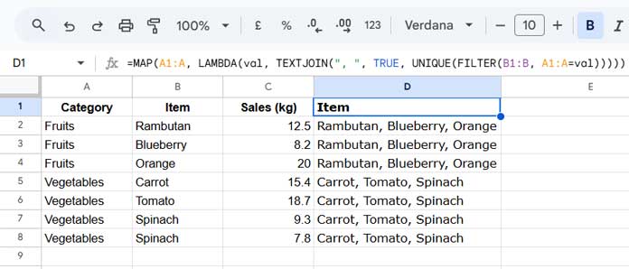
As mentioned earlier, we must add a helper column to the source data. In cell D1, enter the following formula:
=MAP(A1:A, LAMBDA(val, TEXTJOIN(", ", TRUE, UNIQUE(FILTER(B1:B, A1:A=val)))))Where:
A1:Ais the group column (Category).B1:Bis the Item column, which contains the values we want to retain when using QUERY GROUP BY.
Now, use the following QUERY formula:
=QUERY(A1:D, "select A, D, sum(C) where A is not null group by A, D", 1)Compared to the previous formula, here we:
- Expanded the data range to
A1:Dto include the helper column. - Selected and grouped column D.
Result: ✅
| Category | Item | sum Sales (kg) |
| Fruits | Rambutan, Blueberry, Orange | 40.7 |
| Vegetables | Carrot, Tomato, Spinach | 51.2 |
This approach helps you retain all values when using QUERY GROUP BY in Google Sheets.
Helper Column Explained
=MAP(A1:A, LAMBDA(val, TEXTJOIN(", ", TRUE, UNIQUE(FILTER(B1:B, A1:A=val)))))FILTER(B1:B, A1:A=val): Filters the items where the category matches the current row category.UNIQUE(...): Removes duplicate items.TEXTJOIN(", ", TRUE, ...): Joins the items into a comma-separated list, excluding empty values.- The LAMBDA function applies this logic to all categories using MAP.
This helper column is the key to retaining all values or row-level data in QUERY GROUP BY in Google Sheets.


Hi Prashanth,
I have created a Google Sheet, and it contains a database.
I need them into the group by Brand, by ASIN, by MKSU, and the sum of column E to K. Each Brand, each ASIN, Each MSKu need the sum of the totals.
I have got all databases using Query, and I could not be able to get the group-wise.
Kindly help with this. I herewith attached the screenshot for the same along with the Google Sheet with command.
Hi, Saravanan,
I have inserted one QUERY formula in cell A1 in the tab “prashanth kv”.
See if that helps?
If not, please refer to the “Pivot Table 3” tab.
That formula is actually pretty simple to code. If you want that formula explanation, please let me know.
Hi Prashanth, It is very useful and helps a lot.
Hey! Thanks for this nice post.
I was following the tutorial and trying to wrap my head around how SORTN works.
But then I noticed there is an even simpler (well at least easier to understand for my feeble brain) way of achieving the same outcome.
In step number 3, instead of using SORTN to eliminate duplicates, you could just query the resulting array again and do this:
Select Col1, Sum(Col2) Group By Col1.The outcome is the same, because
x + 0 = x.Thanks anyway for this great post, it leads me to solve my problem.
best,
– J
Hey, Jan,
Thanks for your feedback!