Learning essential financial functions in Google Sheets can empower you to make better financial decisions, both personally and professionally. One such crucial function is the PV (Present Value) function.
By learning even one financial function, you’ll find it easier to understand others in this category. If you’re unsure where to start, I recommend the PMT function as a good introduction.
In this tutorial, we’ll explore how to use the PV function in Google Sheets to calculate the present value of a loan or investment.
What Is the PV Function?
The PV function calculates the present value of a series of future payments or a lump sum based on a constant interest rate. In simple terms, it’s the value today of money that will be received or paid in the future.
For example, if you are promised $11,000 a year from now, and the annual interest rate is 10%, the present value of that $11,000 is $10,000. This means that $10,000 today is equivalent to receiving $11,000 one year from now at that interest rate.
PV Function Syntax in Google Sheets
The syntax of the PV function is as follows:
PV(rate, number_of_periods, payment_amount, [future_value], [end_or_beginning])Function Arguments:
- rate: The interest rate per period. For monthly or quarterly payments, divide the annual interest rate by 12 or 4, respectively.
- number_of_periods (Nper): The total number of payment periods. For example, a 5-year loan with monthly payments would have 60 periods (5 years * 12 months).
- payment_amount (Pmt): The payment made each period. If omitted, you must include the future value (FV).
- future_value (FV): The remaining balance or goal at the end of the payment periods. This argument is optional.
- end_or_beginning: Determines whether payments are made at the end (0) or beginning (1) of the period. The default is 0 (end).
Example 1: Lump-Sum Future Payment
Imagine you will receive $11,000 next year, and the interest rate is 10%. The present value of that future amount would be $10,000.
The PV formula would be:
=PV(10%/1, 1, 0, 11000)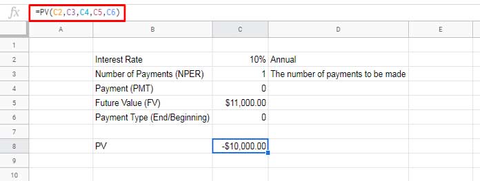
This formula calculates the present value of a future payment of $11,000, assuming an annual interest rate of 10% and a payment period of 1 year.
Example 2: Present Value of Periodic Payments
Now let’s look at how to use the PV function to calculate the present value of monthly, quarterly, and yearly payments over 5 years.
Monthly Payments:
When making monthly payments, divide the annual interest rate by 12. The total number of periods for 5 years is 60 (5 years * 12 months).
=PV(C2/12, C3, C4, C5, C6)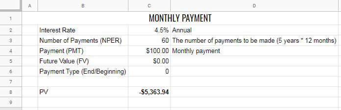
In this case, C2 contains the annual interest rate, C3 contains the number of periods, C4 is the payment amount, C5 is the future value (optional), and C6 is the payment timing (end or beginning of the period).
Quarterly Payments:
For quarterly payments, divide the annual interest rate by 4, and the number of periods becomes 20 (5 years * 4 quarters).
=PV(C2/4, C3, C4, C5, C6)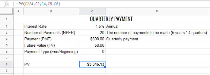
This formula calculates the present value of quarterly payments over 5 years.
Yearly Payments:
For yearly payments, simply use the interest rate as it is without dividing.
=PV(C2, C3, C4, C5, C6)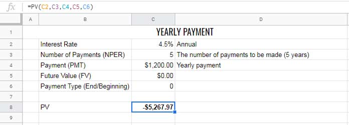
Conclusion
I hope this guide has helped you understand how to use the PV function in Google Sheets. It’s a useful tool for calculating the present value of future payments or investments.
In future posts, I will also compare the PV function with the FV (Future Value) function. Stay tuned for that!
For more tutorials on financial functions, check out my Google Sheets function guide.


